

Comparing experimental conditions: differential expression analysis
Once gene expression data is obtained, one typically wishes to compare one experimental group versus a second one (or more) in order to find out which genes/transcripts change significantly between conditions.
The process is called differential expression analysis.
The goal of differential expression analysis is to perform statistical analysis to discover changes in expression levels of defined features (genes, transcripts, exons) between experimental groups with replicated samples.
Essentially, it aims at comparing the average expression of a gene in group A with the average expression of this gene in group B.
Adapted from this Source
Many tools exist that will perform differential expression analysis. The output of such tools is similar, and essentially revolves around interpreting:
- Fold change:
For a given comparison, a positive fold change value indicates an increase of expression, while a negative fold change indicates a decrease in expression.
This value is typically reported in logarithmic scale (base 2). For example, log2 fold change of 1.5 for a specific gene in the “WT vs KO comparison” means that the expression of that gene is increased in WT relative to KO by a multiplicative factor of 2^1.5 ≈ 2.82. - P-value:
Indicates whether the gene analysed is likely to be differentially expressed in that comparison.
This applies to each gene individually, assuming that the gene was tested on its own without consideration that all other genes were also tested. More on P-value will follow! - Adjusted (or, corrected for multiple genes testing) p-value: The p-value obtained for each gene above is re-calculated to correct for running many statistical tests (as many as the number of genes). In the result, we can say that all genes with adjusted p-value < 0.05 are significantly differentially expressed in these two samples.
How to interpret P-value ?
First, we need to talk about statistical hypothesis testing.
Two hypotheses should be described upon designing an experiment.
- The NULL hypothesis H0: that there is NO difference, for example, of means of weight between two populations of subjects.
- The alternative hypothesis H1: there is difference.
:max_bytes(150000):strip_icc()/null-hypothesis-examples-609097_FINAL-100262e70b70426fb0633304eb2f49f4.png)
Second, we need to talk about the statistical significance of the results of the statistical test.
For that, the significance level, denoted as alpha or α, is defined.
The significance level is the probability to reject the null hypothesis when it is assumed to be true, i.e. concluding that the observed difference of means is the result of a real effect, while in reality it is not.
The significance level of 0.05 indicates a 5% risk of concluding that a difference exists when there is no actual difference.
Once the hypothesis are drawn and the significance level set, we perform a statistical test… and we obtain a p-value.
If the p-value is below the significance level (for example, 0.05), we can reject the null hypothesis in favor of the alternative hypothesis, i.e. we conclude that the observed difference is the result of a real effect.
Example: You study some bacteria and it appears to you that their colonies don’t live more than 65 days.
But you want to check if it is true.
And you want to test your hypothesis at the significance level of 0.05.
So you take a sample of 157 colonies with known life span for each.
You calculate the mean (65.12 days) and the standard deviation (9).
- H0: life spam mean = 65
- HA: life spam mean > 65
It is well known that to test such a hypothesis on the mean of a population there is the z-test.
The test statistic for this z-test is calculated as (each test uses its own formula to calculate the test statistic):
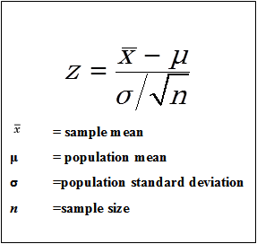
Here:
z = (65.12 - 65) / (9 * sqrt(157)) = 0.167
Each test statistics has a known distribution:
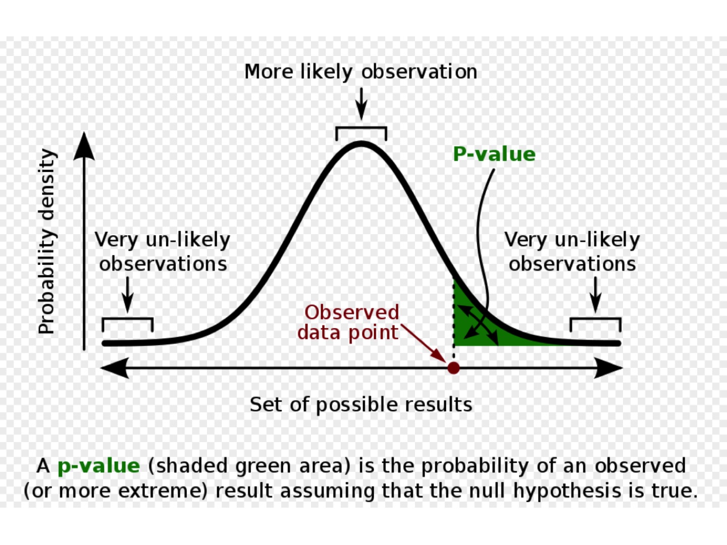
which allows to calculate the p-value, that is, to find the probability of observing a test statistic at least
this extreme when assuming the null hypothesis.
In our case the p-value to obtain the values of z-test statistic greater than 0.167 is equal 0.3936.
Since this is greater than our significance level, 0.05, we fail to reject the null hypothesis (we are NOT in the green zone of the distribution above).
This means that the data does not support the claim that the mean is greater than 65.
Errors can happen in hypothesis testing:
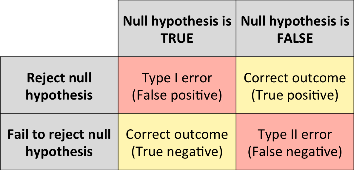
- Type II errors (false negatives): you are missing some real changes!
- Type I errors (false positives): some changes appear to be the result of a real effect while they are not!
Type I errors (false positives) are the most dangerous as they can lead to wrong conclusions.
Why is multiple testing a problem?
Because microarrays and RNA-seq experiments simultaneously monitor expression levels of thousands of genes, there is a multiplicity issue.
Say you have a set of hypotheses that you want to test simultaneously (as for the microarray or RNA-seq assays): as you perform the tests, one day you get a p-value of 0.02. Considering a significance level α of 0.05, this must be significant!
However, if you tried a lot of tests, then you’ve fallen into the multiple comparisons fallacy — the more tests you do, the higher chance you get a p-value < 0.05 by pure chance.
Example of the jelly beans study:
- null hypothesis: jelly beans do NOT cause acne
- alternative hypothesis: jelly beans DO cause acne

Image from this website, original source from xkcd.com
Applying a correction for multiple testing allows you to control the rate of false positive results in your experiment.
The resulting corrected/adjusted p-value is hence more robust than the regular p-value.
Gene selection
It is important to select differentially expressed genes based on the adjusted/corrected p-value (more robust than the p-value).
The Fold change indicates whether a gene is up-regulated or down-regulated.
For example, if we compare 2 experimental groups Wild Type versus Knock Out:
- Fold Change > 0 for gene A means that gene A is more expressed (= up-regulated) in Wild Type compared to Knock Out.
- Fold Change < 0 for gene A means that gene A is less expressed (= down-regulated) in Wild Type compared to Knock Out.
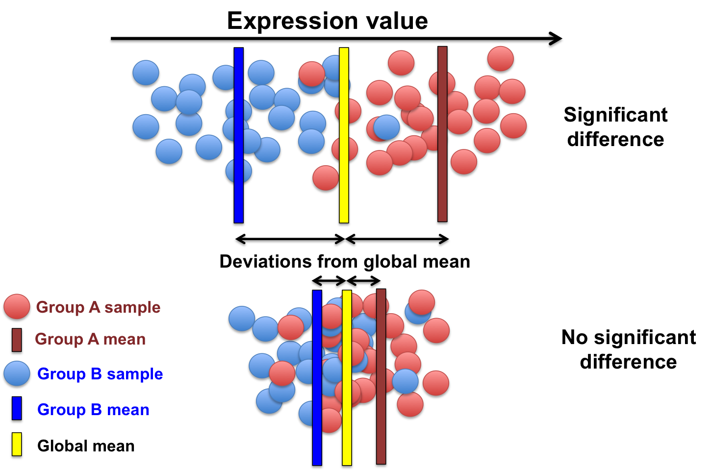
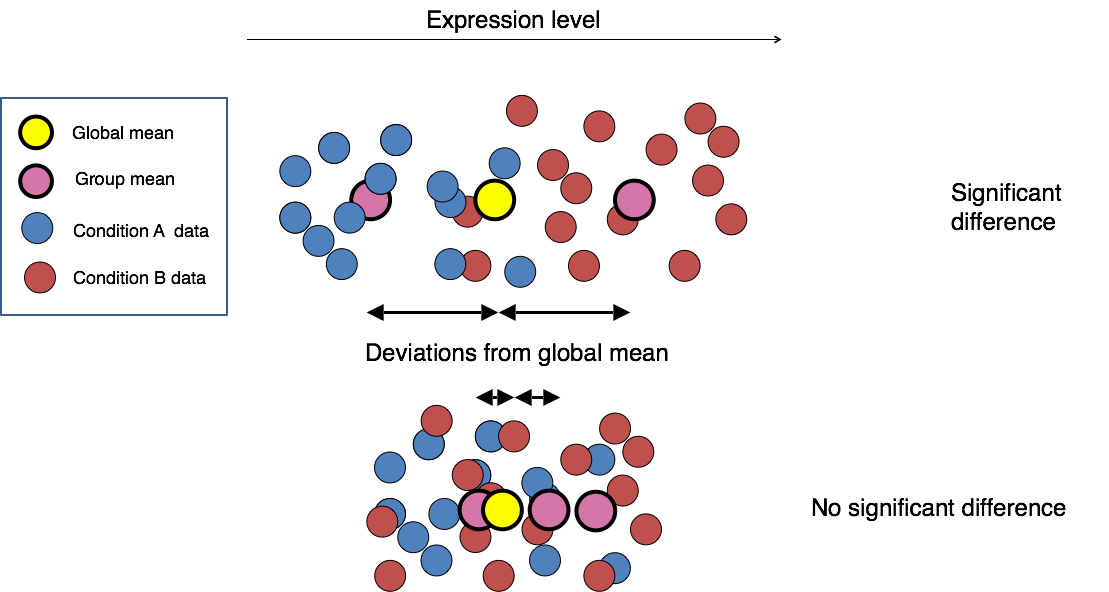
Why the selection shouldn’t be based on fold changes only?
We need to account for variability within experimental groups:
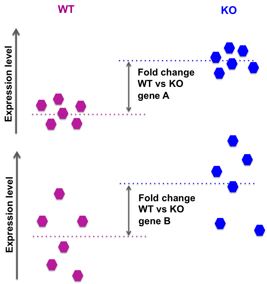
In the picture above: the fold change for gene A and gene B is the same.
However, while the groups average expression levels are similar, we observe a lot more intra-group variability in the case of gene B: we can then expect a lower p-value for gene A than gene B, when comparing WT versus KO.
Analysing differential expression with web-based tools:
Gene expression atlas
The expression atlas holds two types of experiments:
- Baseline (what we have seen in the previous section):
- baseline gene expression for many different tissues and cell types from a wide range of species.
- Differential:
- report genes that are up- or down-regulated in selected experiments.
- selection: the experiment should have at least 2 experimental groups, with 3 biological replicates each and also have a clear control/reference group.
The differential expression results show the differential expression analysis per experiment and per gene.
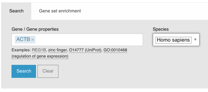
Let’s search per gene.
In the search box on the main page, search ACTB in Homo sapiens:
Click on the Differential expression tab:
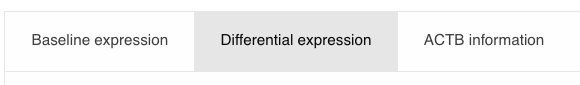
You get, for ACTB, the results of differential expression for all “differential” experiments in gene expression atlas where this gene was found differentially expressed (in Homo sapiens)
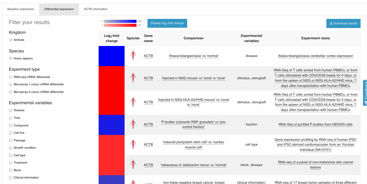
The red corresponds to an up-regulation, and the blue to a down-regulation.
For example, here you can see that in the “RNA-seq of a panel of non-melanoma skin cancer lesions” experiment, ACTB is up-regulated when comparing ‘actinic keratosis’ vs ‘normal’.
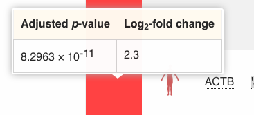
You can mouse over the red box on the left, to see the corresponding fold change and p-value for this specific comparison:
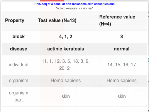
You can also mouse over the comparison name, to get more information such as the number of samples in each experimental group.
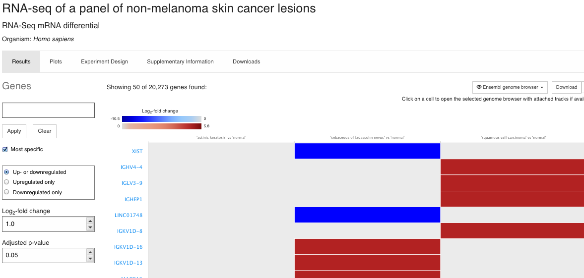
If you want to know more about the experiment itself, you can click on the link in the Experiment name column, and you will be redirected to that specific experiment page.
There you can browse the different panels:
- Results
Up- and down-regulated genes in all comparisons. You can play with log2 fold change and adjusted p-value thresholds, on the left hand panel.
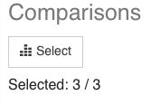
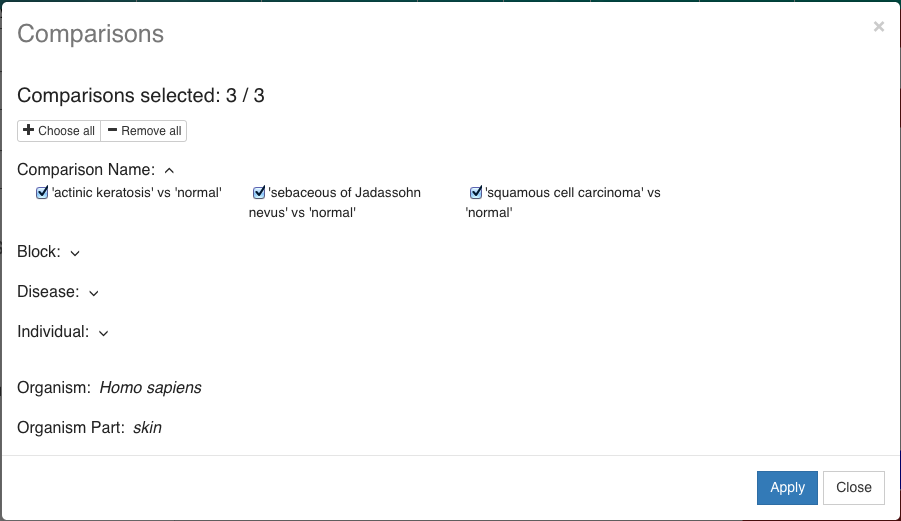
You can also select the comparisons to view:
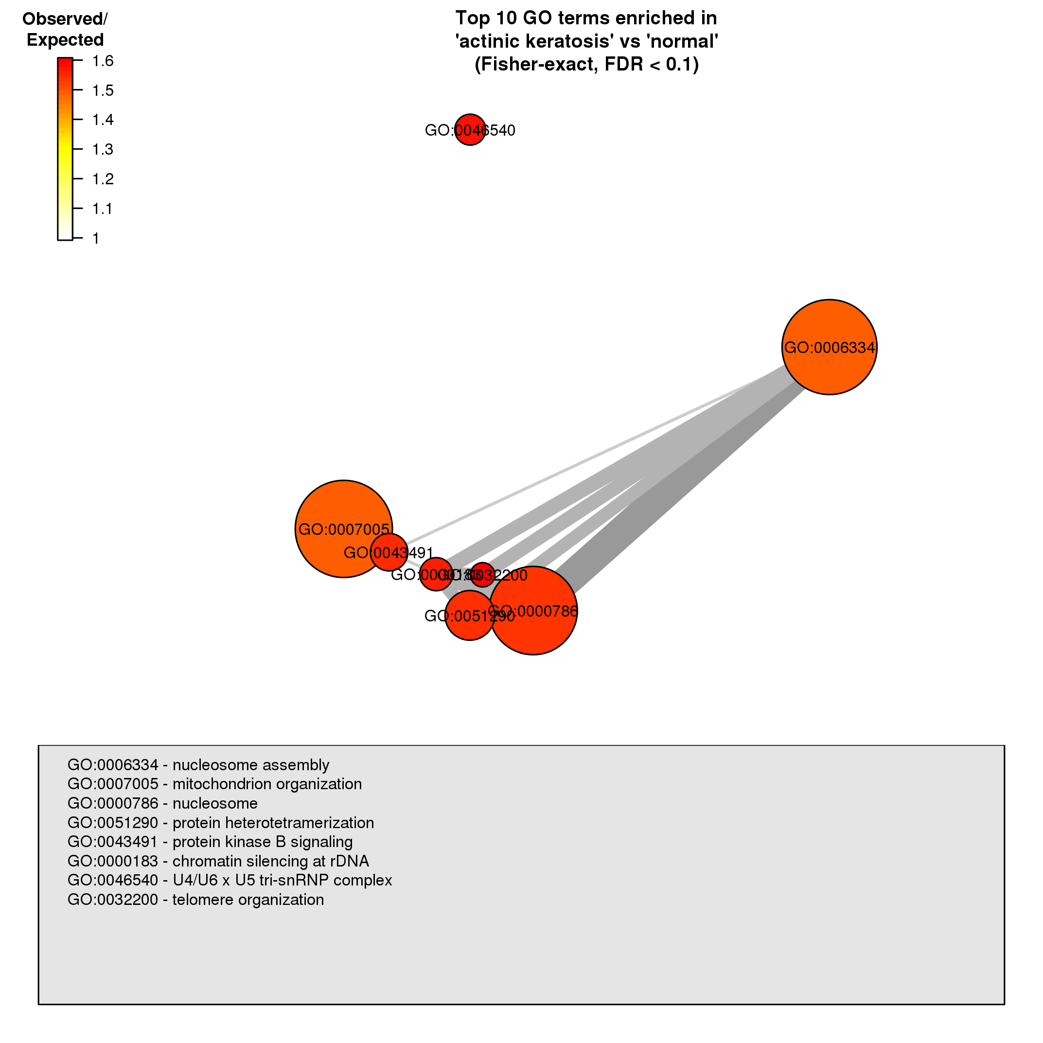
- Plots
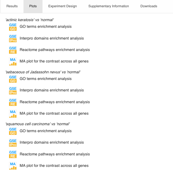
It mainly contains gene enrichment analysis plots, for example, this Gene Ontology enrichment analysis (we will see more of this in the next session).
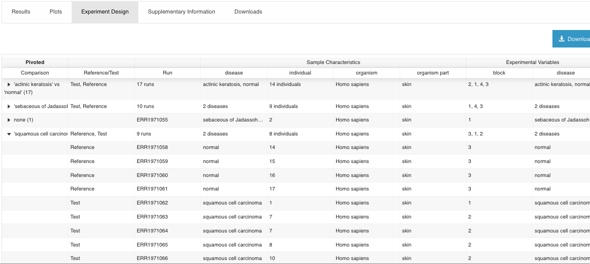
- Experiment Design
It shows what the comparisons correspond to (which samples were selected for each experimental group, etc.).
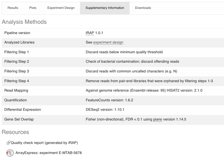
- Supplementary information
The methods for analysing the data are detailed (including tools versions) and you get the access to the data in Array Express (Resources).
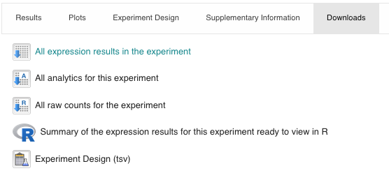
- Downloads
Data available for download:
EXERCISE
- Go to Browse experiments: filter experiments for Saccharomyces cerevisiae.
- Select the RNA-seq experiment from 09-09-2019.
- What is being compared in that experiment? How many comparisons are there?
- What gene(s) has(have) the highest positive fold-change in the ‘14-hour’ vs ‘6-hour’ comparison? What is the corresponding adjusted p-value?
- Do you find genes up-regulated both in the ‘14-hour’ vs ‘6-hour’ comparison AND in the ‘26-hour’ vs ‘14-hour’ comparison?
- How many samples are found in each experimental group (See the Experiment Design tab)?
GEO
Let’s explore one GEO record:
https://www.ncbi.nlm.nih.gov/geo/query/acc.cgi?acc=GSE137345
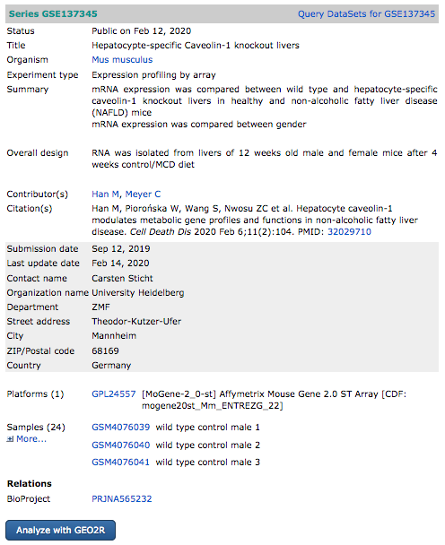
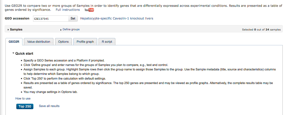
Click on the dark blue button “Analyze with GEO2R”.
“GEO2R is an interactive web tool that allows users to compare two or more groups of Samples in a GEO Series in order to identify genes that are differentially expressed across experimental conditions. Results are presented as a table of genes ordered by significance.
GEO2R performs comparisons on original submitter-supplied processed data tables using the GEOquery and limma R packages from the Bioconductor project. Unlike GEO’s other DataSet analysis tools, GEO2R does not rely on curated DataSets and interrogates the original Series Matrix data file directly.”
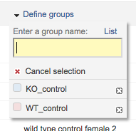
Click on the top of the table “Samples” “Define groups” and define 2 groups: KO_control and WT_control.
Select samples one-by-one and assign to corresponding groups:
- Samples GSM4076039 to GSM4076044 (6 samples) correspond to WT_control
- Samples GSM4076051 to GSM4076056 (6 samples) correspond to KO_control
To do so, select rows that correspond to those samples, then click on the corresponding experimental group in Define groups.
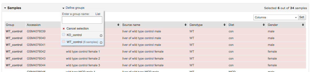
Do the same for the second experimental group.
At the bottom of the page click the blue button Top 250 to see the top 250 differentially expressed genes between KO_control and WT_control.
NOTE that whether the result you obtain depicts KO vs WT or WT vs KO depends on which experimental group you created first!
The first ine you create is the reference: if you first create the WT, then the analysis will show the result as KO vs WT, and vice versa.
The result is one row per gene/probe. Click on this row to see the expression of that gene/probe in each sample:
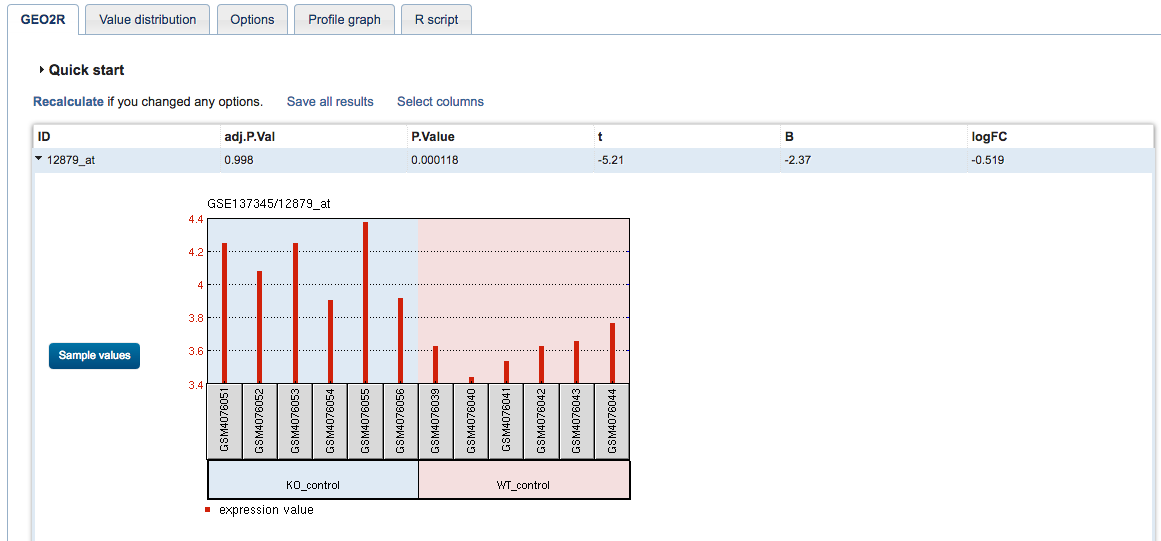
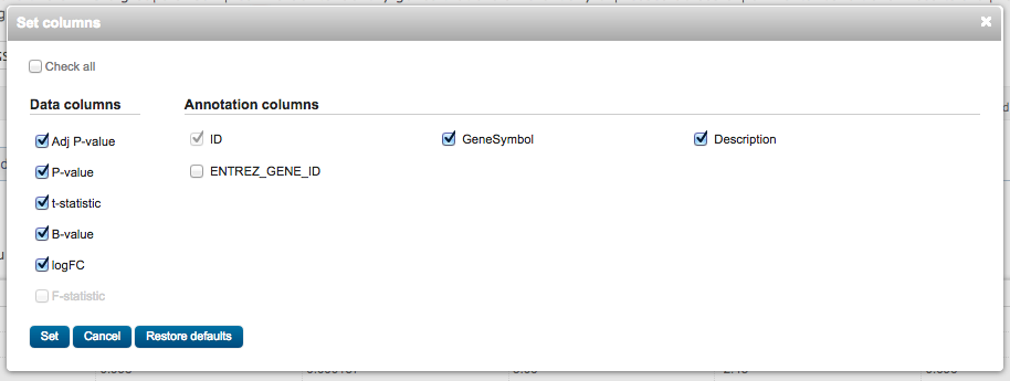
The first column represents the Affymetrix probe ID. To get the more informative gene symbol, click on Select columns and tick GeneSymbol and Description, then Set.
You can look for the Caveolin 1 gene (the one knocked-out in the assay): what are its logFC (log2 Fold Change), P.Value and adj.P.Val (adjusted p-value) ?
We can see that running the analysis with default options not a single gene was found significantly regulated in KO_control versus WT_control (at the FDR adjusted p-value < 0.05).
The GEO page links to the publication where the results of the microarray analysis were published.
In the Minimal overlap between HepCAV1ko and global Cav1 knockout datasets section of the paper, it is written:
“To assess the impact of hepatocyte-specific Cav1 knockout on liver gene expression profiles, we analyzed microarray data of male HepCAV1ko and HepCAV1wt mice liver. We found 1211 genes regulated (p* < 0.05), among them 623 upregulated and 588 downregulated genes*”
This section tells us that the selection was based on the p-value and not on the FDR-adjusted p-value!
How many genes do we find up- or down- regulated, based on p-value < 0.05?
We can save all results, and figure it out:
- Save all results opens a new browser window. Select all the content of the window (CTRL + A) and copy (CTRL + C).
- Next, open an empty Excel (on the training room’s computers, libreoffice) sheet, and paste.
- Finally, you will need to split the data: Data -> Text to columns. Choose the Space as separator.
- Now that the table is properly formatted, filter the P.Value column and answer the previous question: how many genes do we find up- or down- regulated, based on p-value < 0.05?