

The genome
The genome is the genetic material of an organism generally composed of long molecules of DNA. The only exceptions to this definition are the RNA viruses which genome is composed by RNA. The genome comprises regions that are transcribed in RNA and that are not. A portion of the transcribed region is then translated in protein and called coding region, while the rest is named non coding DNA. The DNA of organelles like mitochondria and chloroplasts is also part of the genome of an organism.
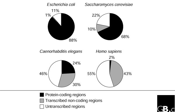 |
| Shabalina SA, et al. The mammalian transcriptome and the function of non-coding DNA sequences. Genome Biol. 2004;5(4):105 |
Genome sequences are usually stored in the FASTA format, while the information about what is encoded in the sequences (aka annotations) are usually stored in the GenBank, GTF or GFF3 formats.
Public resources hosting genomes
Currently there are different databases that host genomic sequences with their annotations:
- ENSEMBL genomes from European Bioinformatics Institute and the Wellcome Trust Sanger Institute.
- GENCODE from a consortium annotating Mouse and Human genomes.
- UCSC genome browser from the University of California, Santa Cruz (UCSC).
- NCBI genomes from National Center for Biotechnology Information, USA.
- GOLD from the DOE Joint Genome Institute.
Some of these online resources also allow displaying information about the genome in a graphical way in the web browser (aka Genome Browser).
Let’s look up for information about the genome of Wuhan coronavirus. Open NCBI genomes in a new tab or window.
Then we can click on Custom Resources –> Viruses and the upper link to go to the NCBI Virus resource.
- How many genomes were sequenced?
- When have they been released?
Let’s click on the first one, with Accession number MN908947. This is the information about this genome stored in the GenBank format.
- What is the genome length?
Scrolling down to COMMENTS, we can see the sequencing technology and the assembly method that were used to obtain this record:
##Assembly-Data-START##
   Assembly Method       :: Megahit v. V1.1.3
   Sequencing Technology :: Illumina
##Assembly-Data-END##
We can extract the genome sequence in FASTA format by clicking on FASTA link on the top left or on Send to on the top right link and then selecting Complete Record –> Choose Destination: File –> Format: FASTA –> Create File Format FASTA.
In this way we retrieve the whole genome sequence that can be displayed in any text editor (it is around 30,000 bases).
>MN908947.3 Wuhan seafood market pneumonia virus isolate Wuhan-Hu-1, complete genome
ATTAAAGGTTTATACCTTCCCAGGTAACAAACCAACCAACTTTCGATCTCTTGTAGATCTGTTCTCTAAA
CGAACTTTAAAATCTGTGTGGCTGTCACTCGGCTGCATGCTTAGTGCACTCACGCAGTATAATTAATAAC
TAATTACTGTCGTTGACAGGACACGAGTAACTCGTCTATCTTCTGCAGGCTGCTTACGGTTTCGTCCGTG
TTGCAGCCGATCATCAGCACATCTAGGTTTCGTCCGGGTGTGACCGAAAGGTAAGATGGAGAGCCTTGTC
CCTGGTTTCAACGAGAAAACACACGTCCAACTCAGTTTGCCTGTTTTACAGGTTCGCGACGTGCTCGTAC
GTGGCTTTGGAGACTCCGTGGAGGAGGTCTTATCAGAGGCACGTCAACATCTTAAAGATGGCACTTGTGG
CTTAGTAGAAGTTGAAAAAGGCGTTTTGCCTCAACTTGAACAGCCCTATGTGTTCATCAAACGTTCGGAT
GCTCGAACTGCACCTCATGGTCATGTTATGGTTGAGCTGGTAGCAGAACTCGAAGGCATTCAGTACGGTC
...
Exercise:
- Investigate the record with Accession number
MT020880released on Feb 5, 2020, by USA.- Using which sequencing technology was this genome sequence obtained?
- Using which sequencing technology was this genome sequence obtained?
- Let’s go back to the NCBI Virus page with the results for coronovirus, sort the results by genome length and select top 10 whole genomes.
Now click the tab on the top right Align to see the multiple alignment of sequences of selected genomes.
What you see is the alignment shown the NCBI Genome Browser.
- Zoom to see the positions 26100-26200. What do you observe?
- Zoom to see the positions 26100-26200. What do you observe?
- Now go back to the genome selection page and click Build Phylogenetic Tree.
- What can you say looking at the country names and release dates?
The genomes stored in public repositories also contain annotations which you can see in the GenBank format under the tab FEATURES. This annotation can be also downloaded in the GFF3 format, using the top right tab Send to -> Complete Record / Choose Destination: File / Format GFF3.
##sequence-region MN908947.3 1 29903
##species https://www.ncbi.nlm.nih.gov/Taxonomy/Browser/wwwtax.cgi?id=2697049
MN908947.3	Genbank	region	1	29903	.	+	.	ID=MN908947.3:1..29903;Dbxref=taxon:2697049;collection-date=Dec-2019;country=China;gbkey=Src;genome=genomic;isolate=Wuhan-Hu-1;mol_type=genomic RNA;nat-host=Homo sapiens
MN908947.3	Genbank	five_prime_UTR	1	265	.	+	.	ID=id-MN908947.3:1..265;gbkey=5'UTR
MN908947.3	Genbank	gene	266	21555	.	+	.	ID=gene-orf1ab;Name=orf1ab;gbkey=Gene;gene=orf1ab;gene_biotype=protein_coding
MN908947.3	Genbank	CDS	266	13468	.	+	0	ID=cds-QHD43415.1;Parent=gene-orf1ab;Dbxref=NCBI_GP:QHD43415.1;Name=QHD43415.1;Note=translated by -1 ribosomal frameshift;exception=ribosomal slippage;gbkey=CDS;gene=orf1ab;product=orf1ab polyprotein;protein_id=QHD43415.1
MN908947.3	Genbank	CDS	13468	21555	.	+	0	ID=cds-QHD43415.1;Parent=gene-orf1ab;Dbxref=NCBI_GP:QHD43415.1;Name=QHD43415.1;Note=translated by -1 ribosomal frameshift;exception=ribosomal slippage;gbkey=CDS;gene=orf1ab;product=orf1ab polyprotein;protein_id=QHD43415.1
MN908947.3	Genbank	gene	21563	25384	.	+	.	ID=gene-S;Name=S;gbkey=Gene;gene=S;gene_biotype=protein_coding
MN908947.3	Genbank	CDS	21563	25384	.	+	0	ID=cds-QHD43416.1;Parent=gene-S;Dbxref=NCBI_GP:QHD43416.1;Name=QHD43416.1;Note=structural protein;gbkey=CDS;gene=S;product=surface glycoprotein;protein_id=QHD43416.1
MN908947.3	Genbank	gene	25393	26220	.	+	.	ID=gene-ORF3a;Name=ORF3a;gbkey=Gene;gene=ORF3a;gene_biotype=protein_coding
MN908947.3	Genbank	CDS	25393	26220	.	+	0	ID=cds-QHD43417.1;Parent=gene-ORF3a;Dbxref=NCBI_GP:QHD43417.1;Name=QHD43417.1;gbkey=CDS;gene=ORF3a;product=ORF3a protein;protein_id=QHD43417.1
MN908947.3	Genbank	gene	26245	26472	.	+	.	ID=gene-E;Name=E;gbkey=Gene;gene=E;gene_biotype=protein_coding
MN908947.3	Genbank	CDS	26245	26472	.	+	0	ID=cds-QHD43418.1;Parent=gene-E;Dbxref=NCBI_GP:QHD43418.1;Name=QHD43418.1;Note=structural protein%3B E protein;gbkey=CDS;gene=E;product=envelope protein;protein_id=QHD43418.1
MN908947.3	Genbank	gene	26523	27191	.	+	.	ID=gene-M;Name=M;gbkey=Gene;gene=M;gene_biotype=protein_coding
MN908947.3	Genbank	CDS	26523	27191	.	+	0	ID=cds-QHD43419.1;Parent=gene-M;Dbxref=NCBI_GP:QHD43419.1;Name=QHD43419.1;Note=structural protein;gbkey=CDS;gene=M;product=membrane glycoprotein;protein_id=QHD43419.1
MN908947.3	Genbank	gene	27202	27387	.	+	.	ID=gene-ORF6;Name=ORF6;gbkey=Gene;gene=ORF6;gene_biotype=protein_coding
MN908947.3	Genbank	CDS	27202	27387	.	+	0	ID=cds-QHD43420.1;Parent=gene-ORF6;Dbxref=NCBI_GP:QHD43420.1;Name=QHD43420.1;gbkey=CDS;gene=ORF6;product=ORF6 protein;protein_id=QHD43420.1
MN908947.3	Genbank	gene	27394	27759	.	+	.	ID=gene-ORF7a;Name=ORF7a;gbkey=Gene;gene=ORF7a;gene_biotype=protein_coding
MN908947.3	Genbank	CDS	27394	27759	.	+	0	ID=cds-QHD43421.1;Parent=gene-ORF7a;Dbxref=NCBI_GP:QHD43421.1;Name=QHD43421.1;gbkey=CDS;gene=ORF7a;product=ORF7a protein;protein_id=QHD43421.1
MN908947.3	Genbank	gene	27894	28259	.	+	.	ID=gene-ORF8;Name=ORF8;gbkey=Gene;gene=ORF8;gene_biotype=protein_coding
MN908947.3	Genbank	CDS	27894	28259	.	+	0	ID=cds-QHD43422.1;Parent=gene-ORF8;Dbxref=NCBI_GP:QHD43422.1;Name=QHD43422.1;gbkey=CDS;gene=ORF8;product=ORF8 protein;protein_id=QHD43422.1
MN908947.3	Genbank	gene	28274	29533	.	+	.	ID=gene-N;Name=N;gbkey=Gene;gene=N;gene_biotype=protein_coding
MN908947.3	Genbank	CDS	28274	29533	.	+	0	ID=cds-QHD43423.2;Parent=gene-N;Dbxref=NCBI_GP:QHD43423.2;Name=QHD43423.2;Note=structural protein;gbkey=CDS;gene=N;product=nucleocapsid phosphoprotein;protein_id=QHD43423.2
MN908947.3	Genbank	gene	29558	29674	.	+	.	ID=gene-ORF10;Name=ORF10;gbkey=Gene;gene=ORF10;gene_biotype=protein_coding
MN908947.3	Genbank	CDS	29558	29674	.	+	0	ID=cds-QHI42199.1;Parent=gene-ORF10;Dbxref=NCBI_GP:QHI42199.1;Name=QHI42199.1;gbkey=CDS;gene=ORF10;product=ORF10 protein;protein_id=QHI42199.1
MN908947.3	Genbank	three_prime_UTR	29675	29903	.	+	.	ID=id-MN908947.3:29675..29903;gbkey=3'UTR
The General Feature Format (GFF) format consists of one line per feature, each containing 9 columns of data, plus optional track definition lines indicated by the first character ”#”.
| Column number | Column name | Details |
|---|---|---|
| 1 | seqname | name of the chromosome or scaffold; chromosome names can be given with or without the ‘chr’ prefix. |
| 2 | source | name of the program that generated this feature, or the data source (database or project name) |
| 3 | feature | feature type name, e.g. Gene, Variation, Similarity |
| 4 | start | Start position of the feature, with sequence numbering starting at 1. |
| 5 | end | End position of the feature, with sequence numbering starting at 1. |
| 6 | score | A floating point value. |
| 7 | strand | defined as + (forward) or - (reverse). |
| 8 | frame | One of ‘0’, ‘1’ or ‘2’. ‘0’ indicates that the first base of the feature is the first base of a codon, ‘1’ that the second base is the first base of a codon, and so on.. |
| 9 | attribute | A semicolon-separated list of tag-value pairs, providing additional information about each feature. |
Exercise: For the NCBI genome with Accession number MT020880 download the annotation file, open it in a text editor and answer the following questions:
- How many genes were annotated for this genome?
- Which genome position encode for the nucleocapsid phosphoprotein?
Whole Genome Sequencing
For years, deciphering the DNA has been a complex procedure. Only around the ’80s the first automatic sequencers became available. Thanks to the long lasting SANGER sequencing the first small genomes became known.
- 1995 The first complete genome was sequenced: Haemophilus influenzae (1.8 Mbp).
- 1996 The first eukariotic genome was sequenced: Saccharomyces cerevisiae (12 Mbp).
- 1998 The first animal was sequenced: Caenorhabditis elegans (103 Mbp).
- 2001 The first draft of the human genome became avialable (3 Gbp).
The Human Genome Project was launched in 1990 and completed 13 years later with an estimated cost of 3 billions dollars. It involved more than 3000 researchers from different institutions and produced the first draft of the human genome (90 percent complete).
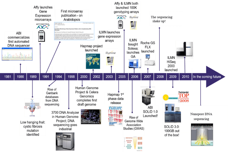
Since then, different companies started to develop automatic methods based on nanotechnology.
- 2005 454 Life science released the first Next Generation Sequencer commercially available. It was bougth by Roche in 2007 and shut down in 2013.
- 2006 Solexa produced the first sequencing by synthesis genome sequencer: the Genome Analyzer. The company was bought by Illumina in 2007 and it is nowadys the most used technology in genomics.
- 2011 Pacific Bioscience start selling its “third generation” sequencer based on single molecule real time sequencing (SMRT). This instrument is able to read a single DNA molecule long up to thousands of bases.
- 2015 Nanopore entered in the market with its own “third generation” sequencer based on sequencing single DNA molecules through nanopores. Recently with this technology scientists were able to sequence reads up to 1 Mb and to analyze the RNA without reverse transcriptase (direct RNA sequencing). With Nanopore it is possible to directly analyze even the chemical modifications of nucleic acids (epi-genomics and epi-transcriptomics).
Genome Assembly
The majority of the platforms produces huge amounts of short sequences called reads. To obtain the final molecules these reads must be assembled using computationally intensive programs. These programs need to compare each sequence against the other and find those that are similar enough to be merged in longer sequence called contigs.
This process can be achieved in different ways, however the most used approaches are often based on the construction and resolution of a De Bruijn Graph.
Currently the introduction of very long reads from Nanopore sequencing is improving dramatically the contiguity of a genome assembly allowing the sequencing complex portions like centromers and telomers. (see https://www.nature.com/articles/nbt.4060).
Genome annotation
After assembly the genomic sequences need to be annotated. The genome annotation is the process of identifying the locations of genome features, such as genes, intron-exon boundaries, regulatory sequences, repeats. A simple method of gene annotation relies on homology based search tools, like BLAST, to search for homologous genes in databases.
After predicting the gene content of a genome, scientists proceed to the next step, that is, inferring possible function of each gene; this process is called Functional Annotation and will be discussed in the next session.
Ab initio methods of genome annotation
These methods rely only on the DNA sequence for the prediction of putative genes. The programs scan the whole genome for detecting DNA portions that have characteristics typical of protein coding or non coding genes. These characteristics are different depending on the organism domain (Bacteria, Eukarya, Archaea) because they differ for the gene structure, for the codon usage and for the presence of peculiar motifs.
| The prokaryotic gene |
|---|
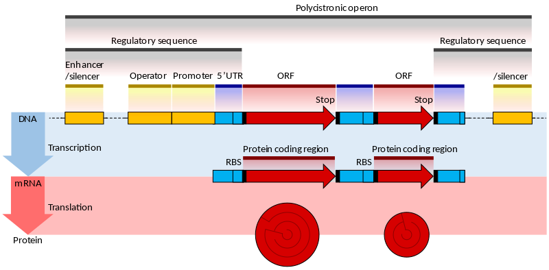 |
| From Wikipedia |
The genes of prokaryotes have well characterized promoter sequences containing known elements, such as the Pribnow box and transcription factor binding sites, that can be identified as markers for downstream genes. The coding sequence (CDS) is a long contiguous open reading frame (ORF), so detecting CDS together eith the promoter is already a good indication of the presence of a real gene. Moreover the bacterial genes are often contained in larger unit called operons.
| The eukaryotic gene |
|---|
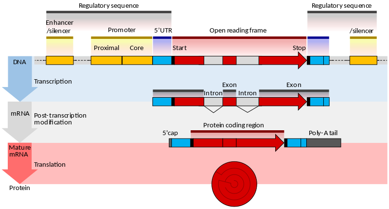 |
| From Wikipedia |
The genes of eukaryotes are more complex, since their promoters are more diverse and the CDS is broken into exons separated by noncoding introns. The programs designed for predicting eukaryotic genes search for additional signals such as:
- presence of CpG islands
- presence of binding sites for polyA tail
- different ORFs
- donor / acceptor splice sites
In most cases programs like GLIMMER and GeneMark for prokaryotes, Augustus and Geneid for eukaryotes create a complex probabilistic model that can be pre-trained on a closest species to better achieve their aim.
The noncoding genes can be searched in a similar way using probailistic models that join both information for the sequence and the RNA secondary structure; for example, the program Infernal that relies on the models stored in the Rfam database allows for detection of RNA gene families.
Empirical methods of genome annotation
Experimental evidences can be used to limit the number of false positives from the ab initio methods and to refine the predictions (for example improving the UTR boundaries). They can also be used to add novel genes that are intrinsecally difficult to find, such as the short genes, the long non coding RNA, etc.
RNA sequences obtained by transcritome sequencing can be used to inform genome annotation by being mapped to the assembled genome. The main drawback of this approach is that in complex organisms only a fraction of genes is expressed at certain time and their expression is also tissue specific.
Genome browsers
Genomic information is stored in databases that can be accessed by the whole scientific community. We already mentioned them previously, saying that they also host web applications able to display the data in a graphical way also known as Genome Browsers, such as
- NCBI Genome Browser (which we already interacted with)
- ENSEMBL Genome Browser
- UCSC genome browser
UCSC Genome Browser
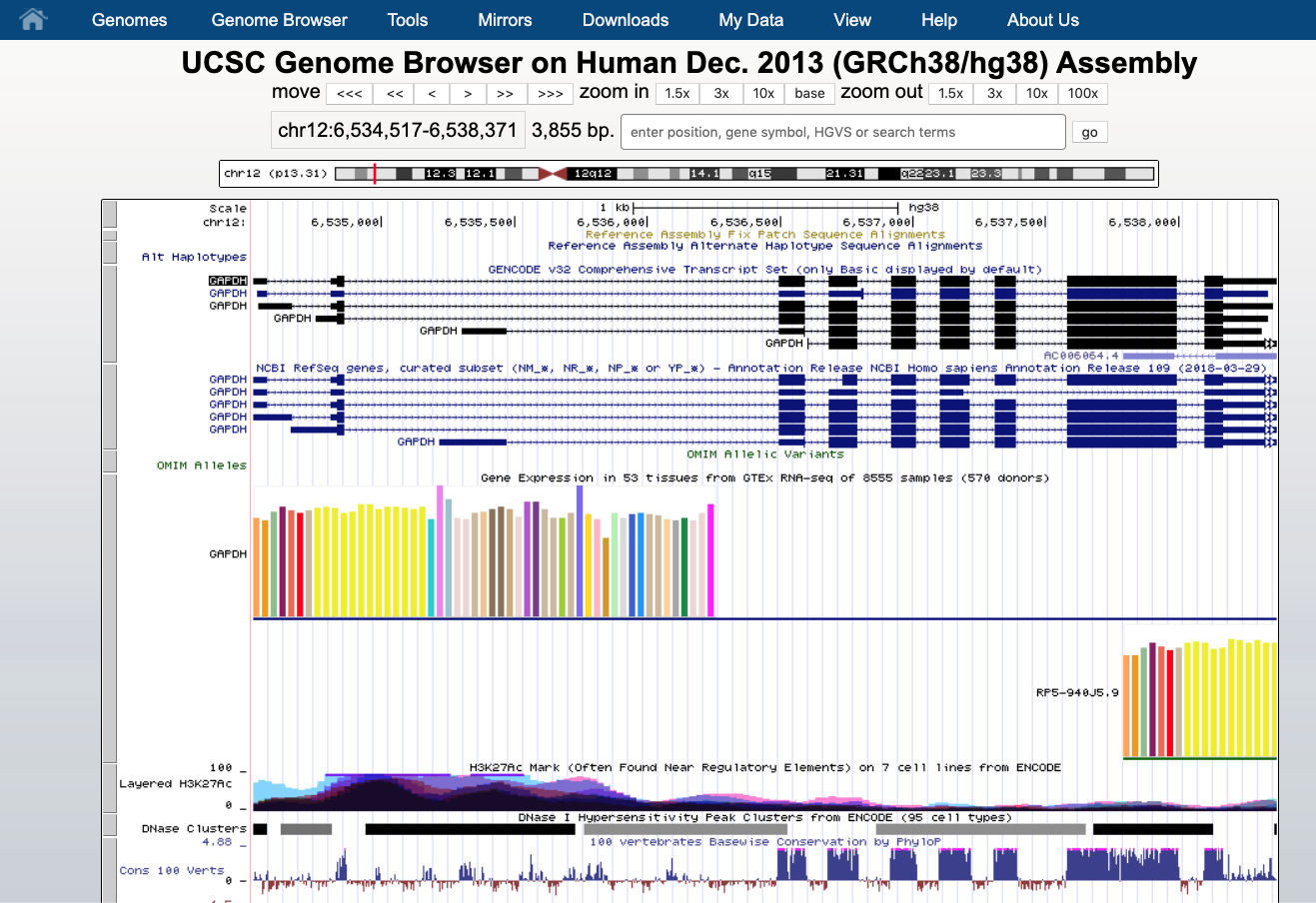
Let’s open the UCSC Genome Browse and search for GAPDH gene in human genome (assembly GRCh38/hg38 - Dec. 2013; this is the most recent available assembly). Specifying the assembly is important since every annotation is likely to have different coordinates among different version of the genome assembly.
We see that the GAPDH gene is located on the chromosome 12 (chr12) at the positions 6,534,517 - 6,538,371. The gene is displayed as a number of boxes (exons) and “arrows” (introns). The arrow direction indicates the gene strand, in this case it lies on the plus strand (5’ -> 3’). Hovering the mouse over the display we can see the positions of each of 9 exons.
Let zoom in to see the sequence of the 9th exon (use the right mouse to do selection).
- What are the exact genome positions of this exon?
- What does the red colored of codon mean?
- And what does the green colored codon mean? (to find out see this help page)
- What does the first letter W in the exon mean?
Every row is a type of annotation. In the example we have:
- GENCODE gene annotation
- NCBI / RefSeq gene annotation
- OMIM allelic variants
- GTEx gene expression
- H3K27Ac histone marks and DNASe clusters from ENCODE
- Conservation among 100 vertebrates
- Common SNPs
- Presence of different families of repeats (Sine, Line etc).
You can click on each row for accessing sub-menus for hiding, showing more, customizing. Below the browser there are different categories of annotations that can be turned on or off depending on the user preference.
You can also add your custom data in different formats by clicking on add custom tracks. As an example you can copy paste the following intervals in BED format:
chr12	6534517	6534717
chr12	6535800	6536000
chr12	6538171	6538371
now they are displayed as black box on the top of the browser. In this way you can display results of your experiments like the ones from a ChIPseq.
Exercise:
Let’s investigate the GAPDH gene a bit more.
- Which of the species shown by default have a difference from human amino acid sequence corresponding to exon 7?
- How many common SNPs does exon 2 contain (expand to the ful view information on SNPs using left mouse hovering it over the left bar)?
- At which positions are these SNPs located (click on each feature)?
- Add the track “TCGA Pan-cancer” from the “Phenotype and Reference” collection of tracks. How many cancer-associated variants were observed in exon 7?
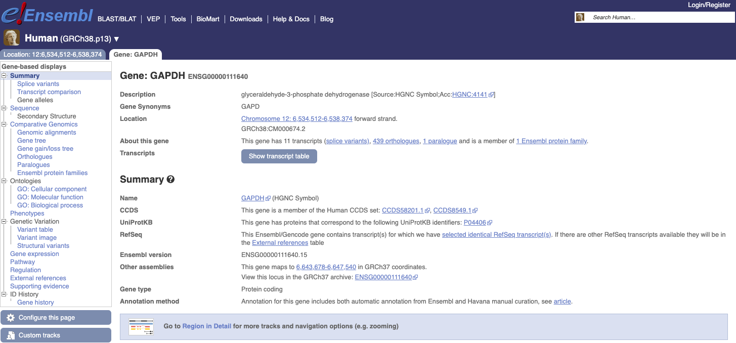
Ensembl Genome Browser
Now let’s move to another genome browser by clicking this link. Let’s search the same gene: GAPDH. You see several results and the “best gene match”. Clicking on it it will show us a new page with information on the gene and below the proper browser.
 |
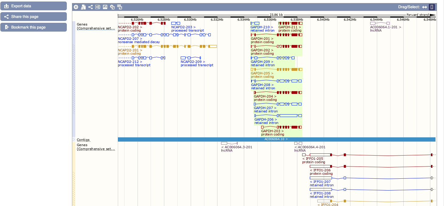 |
A nice help is given clicking on the question mark “?”, while if you click on region detail you are directed on the proper genome browser.
This will bring us to the genomic context with a zoom below on our specific location. Here similarly to UCSC a number of features can be turned on or off by clicking on configure this page.
Exercise:
Let’s investigate the transcripts of the GAPDH gene.
- You can click on Show transcript table to see the list of transcripts and see the “tags” that are associated to each transcript and their meanings. Some transcripts are considered reference transcripts while other are just predicted.
- Have a look at the biotype: not every transcript is coding for proteins. What are the non coding ones?
- From the menu on the left try to quickly access sequence information as exons, cDNA and proteins.