DNA motifs

DNA sequence motifs are short, recurring patterns in DNA that are presumed to have a biological function. Often they indicate sequence-specific binding sites for proteins such as nucleases and transcription factors (TF). Others are involved in important processes at the RNA level, including ribosome binding, mRNA processing (splicing, editing, polyadenylation) and transcription termination.

In the past, binding sites were typically determined through DNase footprinting, and gel-shift or reporter construct assays, whereas binding affinities to artificial sequences were explored using SELEX. Nowadays, they are identified mostly using ChIP-seq experiments.

A DNA motif or pattern is obtained via alignment of DNA-binding sites and is represented as a position frequency matrix (PFM) and “sequence logos” in which a number of stacked nucleotides are placed with a size proportional to their conservation in that position.



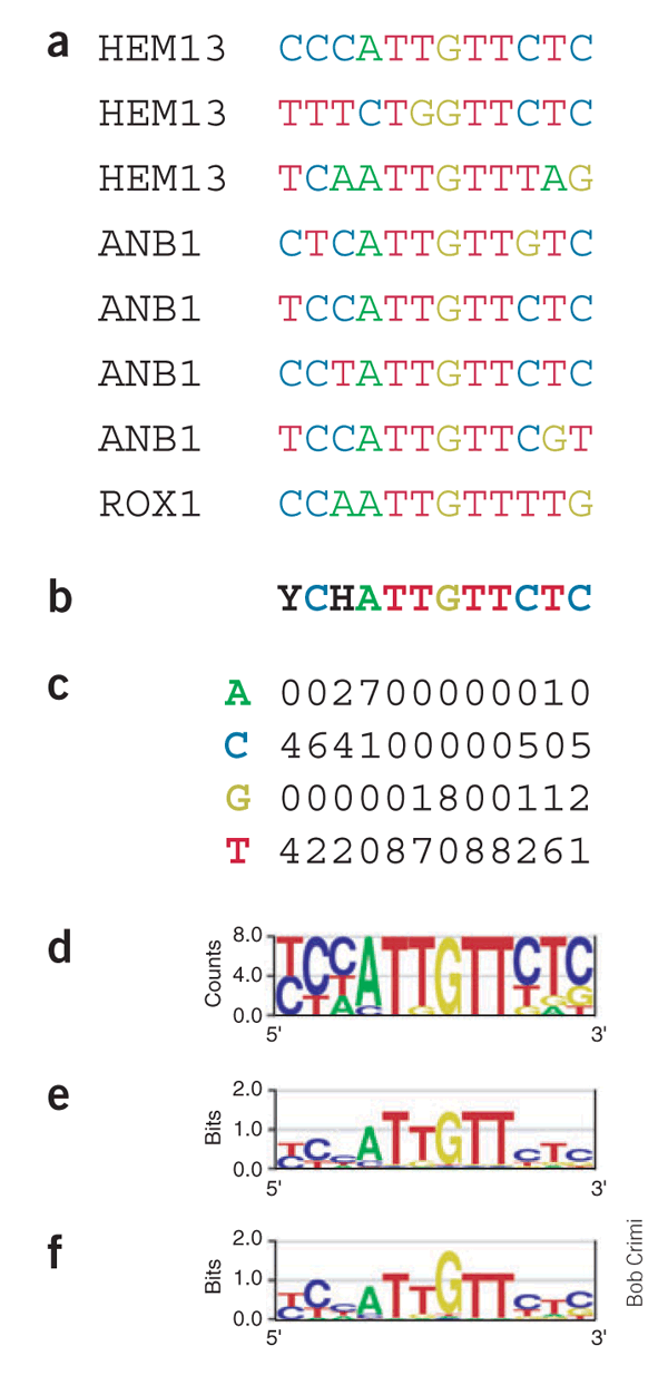(a) Eight known genomic binding sites in three S. cerevisiae genes. (b) Degenerate consensus sequence. (c,d) Frequencies of nucleotides at each position. (e) Sequence logo showing the frequencies scaled relative to the information content (measure of conservation) at each position. (f) Energy normalized logo using relative entropy to adjust for low GC content in S. cerevisiae. From https://www.nature.com/articles/nbt0406-423

(a) Eight known genomic binding sites in three S. cerevisiae genes. (b) Degenerate consensus sequence. (c,d) Frequencies of nucleotides at each position. (e) Sequence logo showing the frequencies scaled relative to the information content (measure of conservation) at each position. (f) Energy normalized logo using relative entropy to adjust for low GC content in S. cerevisiae. From https://www.nature.com/articles/nbt0406-423

For example, the logo (e) is obtained from nucleotide frequencies, applying to each motif position i the formula:

I(i) = 2 + SUM over b of ( f(b,i) * log2(f(b,i) ),

where f(b,i) is the frequency of nucleotide b at position i.

Positions that are perfectly conserved contain 2 bits of information, those where two of the four bases occur 50% of the time each contain 1 bit, and positions where all four bases occur equally often contain no information. Note that for a small sample, the information content will tend to be overestimated, so a small-sample correction needs to be applied. This explains why the central positions of the motif in the logo (e) show an information content of less than 2 bits, even though they are perfectly conserved within the eight known binding sites.

The logo (f) shows the Rox1 binding motif, corrected for the GC-content of S. cerevisiae genomic DNA. In comparison with logo (e), the central G base now carries more information than the flanking A and T bases, reflecting the fact that its occurrence is much more significant in the low-GC genome.

Repositories of known DNA motifs

JASPAR - open source and free collection of motifs as matrices.
TRANSFAC - private collection of eukaryotic transcription factors, genomic binding sites and DNA-binding profiles (there is freely available old version).
CisBP - collects data from >70 sources, including other database such as Transfac, JASPAR, HOCOMOCO, FactorBook, UniProbe, Fly Factor Survey, and dozens of additional publications. In addition to housing these “directly determined” DNA binding motifs, CisBP also includes “inferred” motifs. Inferences are performed by mapping motifs across and within species, using DNA binding domain similarity thresholds established separately for each TF family (see publication for details). In other words, if a mouse TF has a known motif, its human ortholog’s motif can be inferred, provided that the ortholog’s DNA binding domain is “similar enough”.
UniPROBE - a database from the Bulyk lab at Harvard with motifs obtained using the protein‐binding microarray (PBM) technology, either from their own work or from other groups.
PRODORIC - prokaryotic motifs
RegTransBase - prokaryotic motifs

Let’s search JASPAR for Pou5f1. We can see that the mouse motif is slightly larger than the human one (at 5’) but they are quite conserved. Let’s click on the human motif MA0792.1. We can read that the data come from a SELEX experiment.

Now let’s look at another motif, human motif MA1115.1. We see that this motif was derived from the ChIP-seq data. Notice that the binding sites can be downloaded in different formats. For example, in FASTA format:

>hg38_chr1:998688-998698(+)
CGAGGCAAACC
>hg38_chr1:1308251-1308261(-)
TTTTGCAAACG
>hg38_chr1:1752711-1752721(+)
AAATGCAAAAA
>hg38_chr1:1780233-1780243(-)
ATATGCAAAAA
>hg38_chr1:1780247-1780257(-)
TTATGCTAATG
>hg38_chr1:2072658-2072668(-)
aaatgcaaacc
>hg38_chr1:2116080-2116090(-)
gcatgctaatg

...

or in BED format:

chr1	998687	998698	hg38_chr1:998688-998698(+)	.	+
chr1	1308250	1308261	hg38_chr1:1308251-1308261(-)	.	-
chr1	1752710	1752721	hg38_chr1:1752711-1752721(+)	.	+
chr1	1780232	1780243	hg38_chr1:1780233-1780243(-)	.	-
chr1	1780246	1780257	hg38_chr1:1780247-1780257(-)	.	-
chr1	2072657	2072668	hg38_chr1:2072658-2072668(-)	.	-
chr1	2116079	2116090	hg38_chr1:2116080-2116090(-)	.	-
chr1	2116084	2116095	hg38_chr1:2116085-2116095(+)	.	+
chr1	2845689	2845700	hg38_chr1:2845690-2845700(+)	.	+
...
chrX	154790154	154790165	hg38_chrX:154790155-154790165(+)	.	+
chrX	154790202	154790213	hg38_chrX:154790203-154790213(+)	.	+
chrX	154799983	154799994	hg38_chrX:154799984-154799994(+)	.	+
chrX	154918007	154918018	hg38_chrX:154918008-154918018(+)	.	+
chrX	155026565	155026576	hg38_chrX:155026566-155026576(-)	.	-

JASPAR has some other interesting features, such as an application to infer if a protein binds a particular JASPAR motif. Click “Tools” –> “Profile Inference” and use an example sequence.

Or you can display the predicted protein binding within the UCSC and ENSEMBL Genome Browsers by clicking here.

Web applications to create a logo

WebLogo implementing Schneider’s original Sequence Logos as in Figure (e) above.
enoLOGOS provides a variety of options.

Exercise 1.

Obtain a sequence in FASTA format of the human YY1 protein. You can use NCBI or UniProt website. NOTE: Consider the longest isoform.
Find in JASPAR DNA motif(s) this protein is predicted to bind. The tool to use is here. Select the motif obtained using ChIP-seq.
Q1. What is the length of the motif (in base pairs).
Q2. Which positions of the binding site (looking at the JASPAR logo) are conserved?
Q3. From which type of the experiment the binding sites to build this motif were obtained?
Q4. How many sequences were used to build the motif?
Q5. Obtain sequences of binding sites (download FASTA file) and build a logo, using WebLogo for the first 20 sequences. (TIP: You might need to change the parameter “Logo range” and “Logo size” to clearly see the logo for the binding sites.). Compare this profile with one stored in JASPAR. Which pisitions of the profile are conserved?
Q6. Now build the logo for the last 10 sequences and compare it with the JASPAR profile. How is it different from the JASPAR’s one and that one you built for the first 20 sequences? Which positions are conserved in this profile?

DNA motif discovery

You can also be interested in discovering novel and known motifs from your own experimental data or to see if in particular conditions there are different motifs. In case of searching for known motifs (that are in databases) you might find a protein that is competing for the same positions as the protein you study or acting in a complex with your protein.

To address these tasks, there is a number of tools, some of which are also available as online web app. For example, the MEME suite includes motifs from many databases and has tools that can be used to discover motifs de novo in sets of sequences, to compare motifs to each other and to search sequences for matches to motifs.

Exercise 2. Using GOMo program of the MEME suite (see Motif enrichment) identify top five Gene Ontology terms associated with human genes which promoters contain the JASPAR motif for the human YY1 transcription factor. (TIP: Save the JASPAR motif in the MEME format first.)

We will use the MEME motif discovery tool to discover DNA motifs in the Suz12 DNA-binding regions on chromosome Y of the mouse genome, obtained in the ChIP-seq experiment discussed before.

For that, we first need to obtain the DNA sequences of the ChiP-seq peaks located on chrY. We can do it using the UCSC Genome Browser as follows:

Let’s first download (again) a list of the Suz12 protein binding regions obtained from the ChIP-seq experiment and provided in the BED file GSE41589_Suz12_BindingSites.txt.gz in GEO entry “GSE41589”.
Open the UCSC genome browser. Select “Mouse”. Select the assembly “mm9” and click “GO”. Add Custom track by uploading the file GSE41589_Suz12_BindingSites.txt.gz.
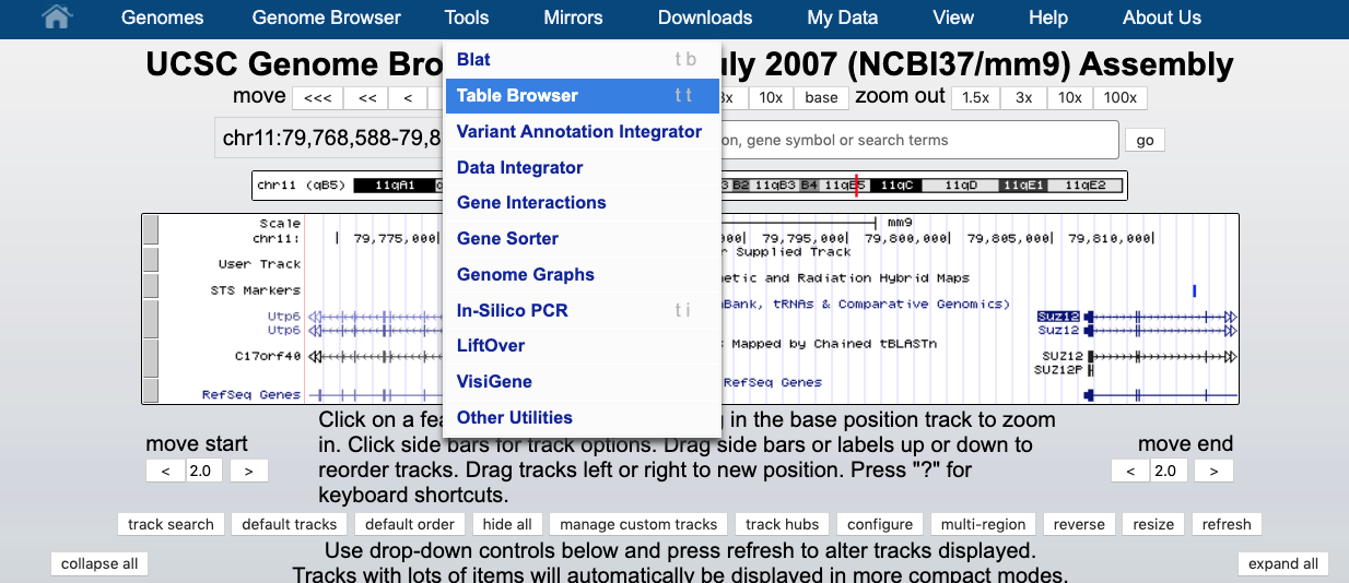
To obtain sequences of the regions specified in the custom track, on the top panel of the Browser window select TOOL -> TABLE BROWSER as shown below.

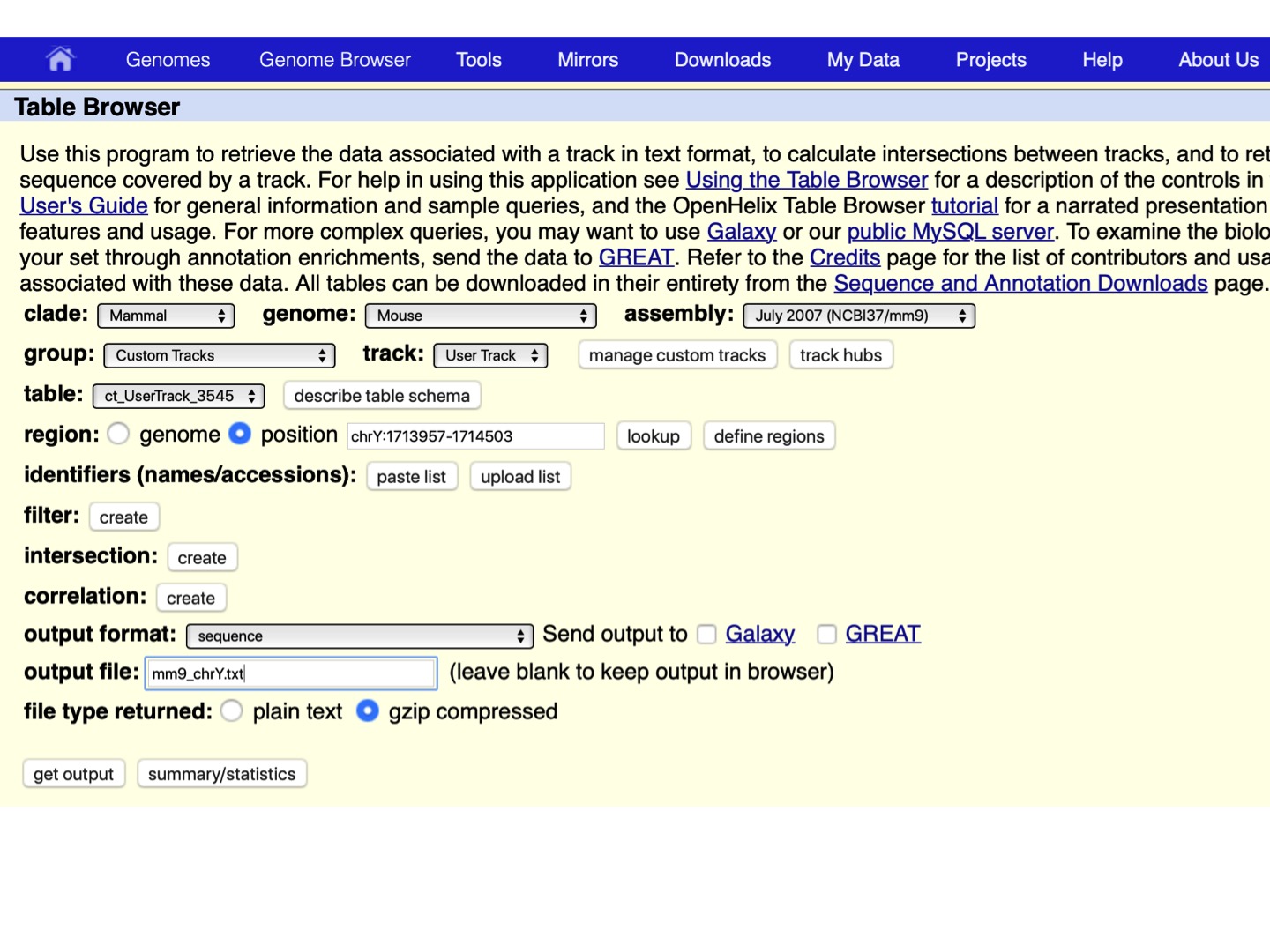
Choose region -> position: chrY, output format: sequence, define a name in the output file (e.g., mm9_chrY.txt), and click get output, as shown below.

Let’s open the downloaded file of DNA sequences corresponding to the ChIP-seq peaks identified on chrY:

>mm9_ct_UserTrack_3545_0 range=chrY:1713957-1714503 5'pad=0 3'pad=0 strand=+ repeatMasking=none
CAGAATGTGACTCAGGTCATCAGGTCATTTCGGTAGGGAATTAATTTTGG
GTTTCTAGGAGGCCATATGAAAAGGTAAAGCCTAGATGCTGAAAGTTTCT
GAGTCCAACTAGGGAAGGAACCAGCATGAGAGGGGTTCTATGATGTAAGC
TGAACTAGAGTGATGTTACAGAGCACTGGTCAGGGGTTTGCACATCTATT
CCACTTGGAGGCGCTAGAATCCCTTGAAGGTGGGTGGGTACTACTATGTT
TGCAGTAGTGTGTAAAAGCCAGGTCAGCTCCTGAACCACAAAGTTGTTCC
ATAGGCTTTTGGTGCCTGGTCTGTATCAGAAGACAGAATCTTGACGACTA
GGACATTTTCTTTGAGAAAGTACATTTATGAAGTAACTGGGACCCTCATA
GCTCCAGAAAGCTAAAAGTTTTCCCTCCTACAGTGAGTAACTGTACATTC
TAATTTCTCCCATGTTTGGGAGCTAGGAGGATGGATGGTCTAGGTTAGTG
GATCTTCTGAATTTATTATCCTTGCTAACAATATCTCATTCACAATT
>mm9_ct_UserTrack_3545_1 range=chrY:1788288-1788617 5'pad=0 3'pad=0 strand=+ repeatMasking=none
TTCAGTTACTGCATTCTACTGAATTTCGGGATACTTGGCCTGCCTTGCCC
TTTGAAGCCTCACTGTGGATTTCGTGGCAAAAATTTTTCCTGAAACATTC
AATGAAGCCAAATTCTTGACCTTTGTCGTGCTAGGATTCTGCAGTGTCTA
TGTCACCTTCCTCCAAGTCTCACATAGCACTAAGGGCATGGTCATGGTTG
CTGTAGAGGTCTTCTCAATCTTGGCATCCAGTGCAGAGATGCTTGGATGC
ATCTTTACACCCAAGATCTATATCATTGAAATAAGACCAGACTTAAATTC
TATCCAAGGTTTCAGATAGAAGTCAGATAT
>mm9_ct_UserTrack_3545_2 range=chrY:2488606-2489040 5'pad=0 3'pad=0 strand=+ repeatMasking=none
TAAAAGATGTTAAAGAGGAAGGCCTCCCTGTAGGAGGACCAAAAGTGTCA
ATTGAAATGCTCCACCAAGATGTCTAAAAATCTGGCCCAACATAGAGACT
ACTAAACCTGCTGATATGAGGCCTCCAACACACGTACAGAAGAGAATTTC
TGGGAGGAGGACTCTACACTTCCCCTCTCCCCACTGGAGGGCATTTCATC
TAATGTCTCTCCCTTTGAGTCCTGAGAGTCTCTCACATCCCAGGTCTTTG
GTATATTCTAGAGGGTTTTCTCACCTCCTACCTCACAAAGTTGCCTGTTT
CCATTCTTTTTGCTGGTCTTCAGCTCTTCAGTCCTGTTTCCCAACCCCCA
CAGTTCCCGATCAAGTTTCTCTCTTCCCCTCTTTGTACCCTTTCACAGCC
AGGTCTCTCCCTCCAACTCCCTGTAGTAATTTTTT
>mm9_ct_UserTrack_3545_3 range=chrY:2792514-2793303 5'pad=0 3'pad=0 strand=+ repeatMasking=none
GTAATTCACAGACCACATGAAGGTCAAGCAGAAGGAAGATGAGAGTGTGG
GTGTTTCAATCCCTCTTAGAATGGGGAACAAAATACTCCTTGGAAAAAAT
ATGGAGACAAAGTGCAGAGCAGAGACTGAAGGAATAACTATCCATTGTCA
GCCCAACCTGTGGATCCATCCCATATACAGACACCAAACCCAATCACTAT
TGTGGATACCAACACGTGCTTGCTGACAGGAGCCAAATATGGCTATCTCC
TGAGAGGCTCAGCCGTTTATTGGCAAGAAAAGAGGCTGATGCTCACAGAC
AACTATCAGACATATCATGGGGTCCCCAGTAGACGAGTTACAGGAAGAAC
TGAAGGAGCTGAAGTTGCTTATAACTGAAGCAACCTTATAGGAAGAACAA
CAATATGAACCAACCAGACTGTACAGAGCACCTAGGGACTAAACACCAAC
CCATGGTTCCAGCTGCATATATAGCAGAGTATGACCTTGTCAGACATCAG
TGGGAGGAGAGGTCCTTGGTCCTGTGAAGGCTTGATTCCCCAGTGTAGGC
ATGTACCAGGGTGGGGAGGGTAAAATGGGTGGATGGAGGAAAACCCTCGT
AGAAACACAGAGAGGGTAAATGGAATAGGGATTATCTGGGGTGAAACAAA
GAAAGGACTAATATTTGAAATGTAAAGAAAGGTAATATCTAGTAAAAATA
AATAAATAAATAAATAAACAAATAAAATAAAAATAGTTACAAAACACTAC
ATATAAAAAGAATAATTCACTATGATGTCATACAGTATAT
>mm9_ct_UserTrack_3545_4 range=chrY:2862963-2863751 5'pad=0 3'pad=0 strand=+ repeatMasking=none
TTTACATTTCAAATATTAGTCCTTTCTTTGTTTCACCCCAGATAATCCCT
ATTCCATTTACCCTCTCTGTGTTTCTACGAGGGTCTTCCTCCATCCACCC
ATTTTACCCTCCCCAACCTGGTTCATGCCTACACTGGGGAATCAAGCCTT
CACAGGACCAAGGACCTCTCCTCCCACTGATGTCTGACAAGGTCATACTC
TGCTATATATGCAGCTGTAACCATGGGTTGGTGCTTTGTCCCTGGGTGCT
CTGGACAGTCTGGTTGGTTCATATTGTTGTTCTTCCTATAAGGTTGCAAT
CCCATTCAGCTCCTTCAGTTCTTCCTGTAACTCGTTTACCCCATGATCAG
TCTGATAGTTGTCTGTGAGCATCAGCCTCTTTTCTTGCCAAGAAATGGCT
GAGCCTCTCAGAAGATAGCCATATTTGGCTCCTGTCAGCAAGCACGTGTT
GGTATCCACAATAGTGATTGGGTTTGGTGTCTGTATATGGGATGGATCCA
CAGGTTGGGCTGACAATGGATAGTTATTCCTTCAGTCTCTGCTCTGCACT
TTGTCTCCATATTTTTTCCAAGGAGTATTTTGTTCCCCATTCTAAGAGGG
ATTGAAACACCCACACTCTCATCTTCCTTCTGCTTGACCTTCATGTGGTC
TGTGAATTACATTTTGGATATTCTGAATTTTTAGAATAATATCCCTTTAT
CAGTGAGGGTGTACCATGTTTGTAATTTTGGGATTGGGTTACCTCACACA
GAATGATATATTTTATATCCTTCCATTTGCCTGTGTATT

We can see that the file contains five sequences, each corresponding to the ChIP-seq peak on chromosome Y.

We can now go to the MEME program to identify common DNA motifs in these five peaks. And upload the uncompressed file of downloaded peak sequences, mm9_chrY.txt.

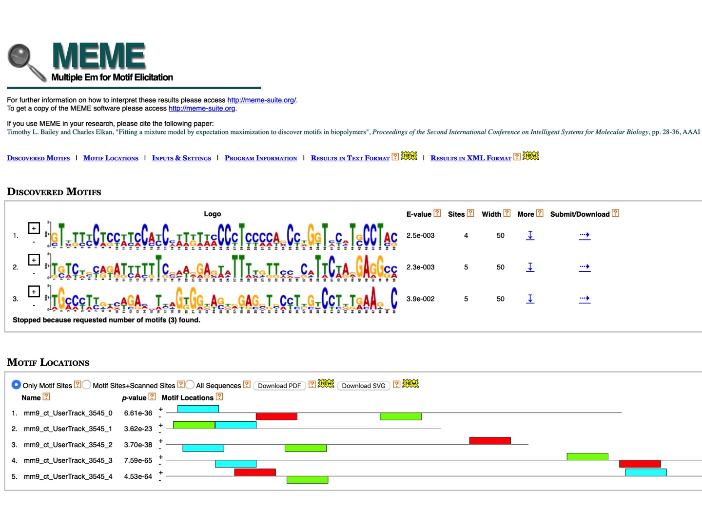
We see that MEME found 3 motifs (as many as were defined in the parameter list, by default). From here, we can submit any motif directly to other programs of the suite or download them in the MEME format and analyze using other external programs.

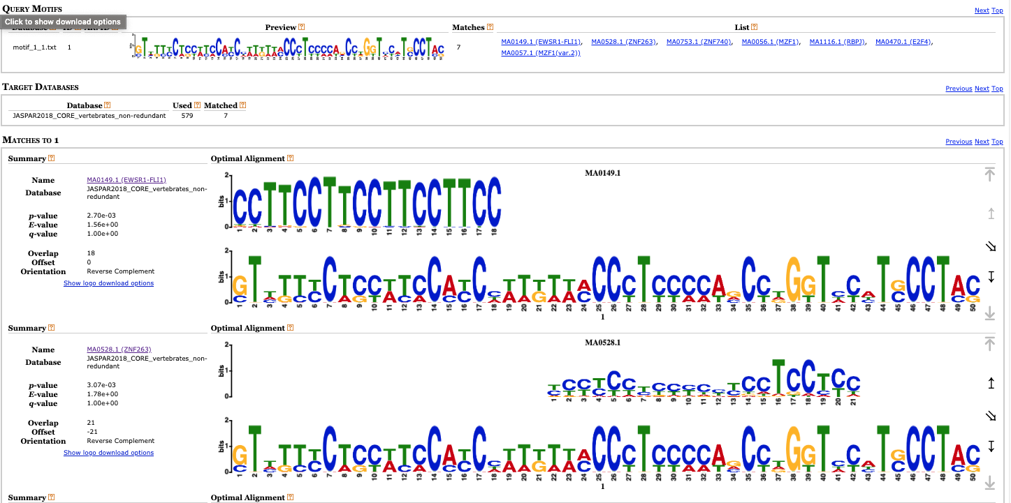
For example, we can submit the first motif to the tool TomTom that allows to compare our motifs with those that can be found in the DNA motif databases. Let’s select target motifs from JASPAR CORE and UniPROB mouse. We can see that among different results we got matching profiles for TFs with DNA binding zinc finger domains, and it is known that Suz12 is a protein containing a zinc finger domain.

Other tools in the MEME suite allow to scan whole genomes for finding positions compatible with the motif matrix and the closest genes (i.e., the ones that are likely under control of that transcription factor).

You can try some of those tools, for example, Fimo that produces a list of positions matched by the motif or T-Gene that predicts regulatory links between genomic loci and genes.

Exercise 3.

A core promoter of a gene is a short sequence encompassing ˜50 base-pairs (bp) upstream and ˜50 bp downstream of the TSS. The core promoter serves as a binding platform for the transcription machinery, which comprises Pol II and its associated general transcription factors (GTFs). Core promoters are sufficient to direct transcription initiation6, but generally have low basal activity, which can be further suppressed by chromatin or activated by often more distally located regulatory elements called enhancers https://www.ncbi.nlm.nih.gov/pmc/articles/PMC6205604/.

The TATA box, the first core promoter element to be identified (in 1978), was biochemically found to be located 20–30 bp upstream of the transcription start site (TSS). The TATA box is found in only about 5–7% of eukaryotic promoters. https://www.ncbi.nlm.nih.gov/pmc/articles/PMC4340783/

In this exercise, we will use the UCSC Genome Table to extract sequences of the core promoters of the following human genes known to contain the TATA-box:

UCP3 
UGT1A7
RMRP
CYP2A6
MBL
GH1
NOS2A
PRTN3
ABCA1

We will use the following UCSC table and setup:

assembly: hg19
group: Genes and gene prediction
track: UCSC genes
table: knownGene
region: genome
output format: sequence

Here are the corresponding gene names to use with that specific UCSC table:

uc001our.3
uc002vut.3
uc003zxh.2
uc002opl.4
uc001jjt.3
uc002jdi.3
uc002gzu.3
uc002lqa.1
uc004bcl.3

Output genomic sequences, selecting 60 bases in promoter/upstream and 0 bases donwstream of transcription start site and one FASTA record per gene.

Cut and paste these sequences into MEME program, selecting for “Input the primary sequences” –> “Type in sequences”. Use advanced options in MEME to search for motifs of size from 4 to 10 and only on a given strand.

Q1. If you found the TATA box, identify the range of positions upstream of TSS it is located in the given promoters.

Proceed to submit this motif to TomTom to search it in the JASPAR CORE and UniPROBE Mouse collection of motifs. Investigate the best matching motif in JASPAR.

Q2. How many protein binding sequences were used to build this JASPAR motif?

Q3. Which protein binds the TATA box?