

The genome
The genome is the genetic material of an organism generally composed of long molecules of DNA. The only exceptions to this definition are the RNA viruses which genome is composed by RNA. The genome comprises regions that are transcribed into RNA and others that are not. A portion of the transcribed region is then translated into protein and called coding region, while the rest is named non-coding DNA. The DNA of organelles like mitochondria and chloroplasts is also part of the genome of an organism.
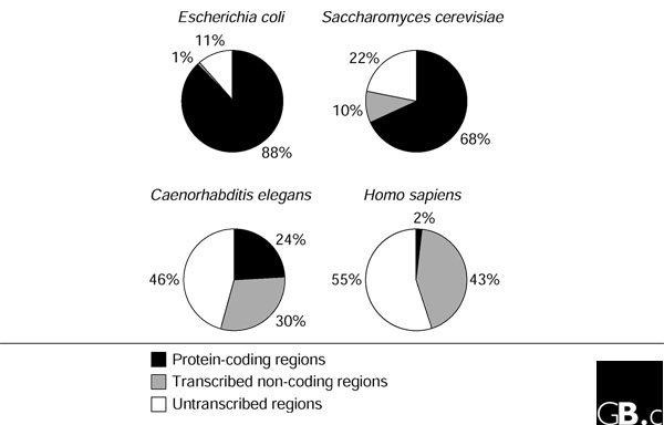 |
| Shabalina SA, et al. The mammalian transcriptome and the function of non-coding DNA sequences. Genome Biol. 2004;5(4):105 |
Whole Genome Sequencing
For years, deciphering the DNA has been a complex procedure. Only around the ’80s the first automatic sequencers became available. Thanks to the long lasting SANGER sequencing the first small genomes became known.
- 1976 The first complete viral genome was sequenced: Bacteriophage MS2 (3,569 bp)
- 1995 The first complete genome was sequenced: Haemophilus influenzae (1.8 Mbp).
- 1996 The first eukariotic genome was sequenced: Saccharomyces cerevisiae (12 Mbp).
- 1998 The first animal was sequenced: Caenorhabditis elegans (103 Mbp).
- 2001 The first draft of the human genome became available (3 Gbp).
The Human Genome Project was launched in 1990 and completed 13 years later with an estimated cost of 3 billions dollars. It involved more than 3000 researchers from different institutions and produced the first draft of the human genome (90 percent complete).
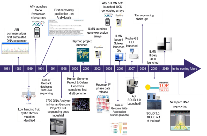
Since then, different companies started to develop automatic methods based on nanotechnology.
- 2005 454 Life science released the first Next Generation Sequencer commercially available. It was then bought by Roche in 2007 and finally shut down in 2013.
- 2006 Solexa produced the first sequencing by synthesis genome sequencer: the Genome Analyzer. The company was bought by Illumina in 2007 and it is nowadays the most used technology in genomics.
- 2011 Pacific Biosciences (PacBio) starts selling its “third generation” sequencer based on single molecule real time sequencing (SMRT). This instrument is able to read a single DNA molecule long up to thousands of bases.
- 2015 - 2020 Nanopore entered in the market with its own “third generation” sequencer based on sequencing single DNA molecules through nanopores. Recently with this technology scientists were able to sequence reads up to 1 Mb long and to analyze the RNA without reverse transcriptase (direct RNA sequencing). With Nanopore it is possible to directly analyze even the chemical modifications of nucleic acids (epi-genomics and epi-transcriptomics).
- 2015 - 2020 BGI Group start produceing a number of sequencing platform able to compete with Illumina for cost and quality of produced reads like the DNBSEQ-T7 that can generate 1-6Tb of high quality data per day.
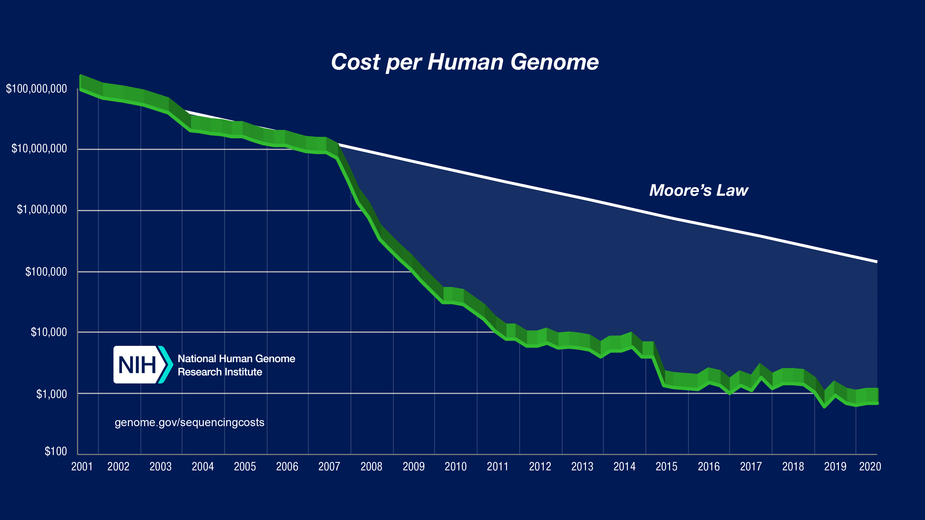
The cost of sequencing a human genome decreased faster than the Moore Law, that predicts that the complexity of a chip double each 18 or 24 months. Currently we have another problem that is related to storage capacity and computational power!
Genome Assembly
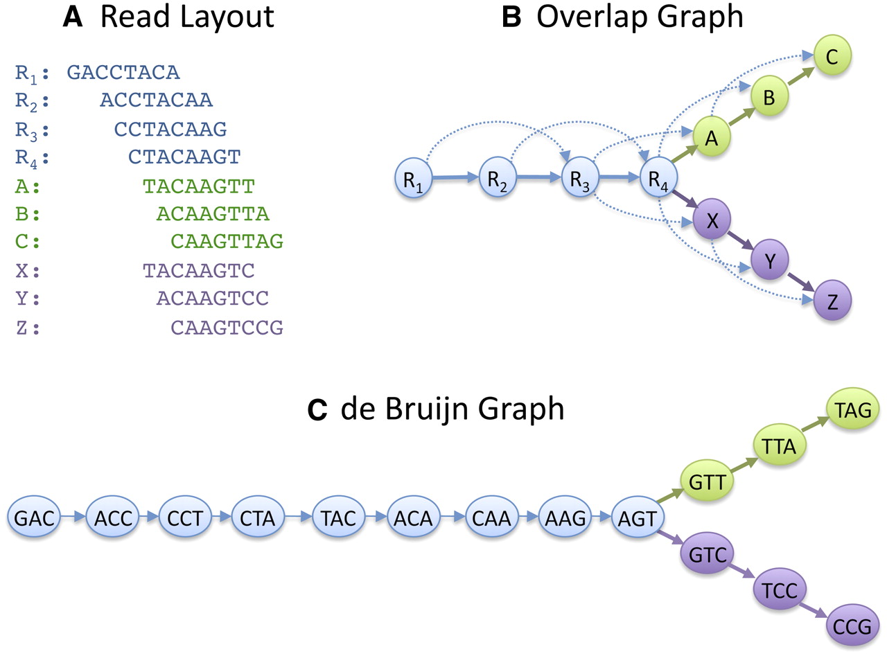
The majority of the platforms produces huge amounts of short sequences called reads.
To obtain the final molecules these reads must be assembled using computationally intensive programs.
These programs need to compare each sequence against the other and find those that are similar enough to be merged into longer sequences called contigs.
This process can be achieved in different ways, however the most used approaches are often based on the construction and resolution of a De Bruijn Graph.
 |
| Schatz MC et al. Assembly of large genomes using second-generation sequencing. Genome Res. 2010 Sep;20(9):1165-73. |
Contigs can be then joined together generating the scaffolds and these can be grouped together up to reconstructing the final chromosomes. This can be achieved using experiments that give long-range information such as mate-pair sequencing with long inserts, the Chromosome conformation capture, the sequencing of libraries of fosmid vectors etc.
Currently the introduction of very long reads from Nanopore sequencing is improving dramatically the contiguity of a genome assembly allowing the sequencing complex portions like centromers and telomers. (see this article).
Genome sequences are usually stored in FASTA format, while the information about what is encoded in the sequences (aka annotations) are usually stored in the GenBank, GTF or GFF3 formats.
Currently there are different public databases that host genomic sequences with their annotations (listed at the end).
As an example let’s look up for information about the genome of the SARS-Cov-2 virus
This information is stored within the NCBI database, in the section NCBI genomes.
We can click on Custom Resources –> Viruses and the upper link to go to the NCBI Virus resource.
Here we can see more than 86 thousands sequences and one RefSeq Genome, that is the first one that was made available. We can inspect it by clicking on the links so as to retrieve all the important informations.
We can check the genome size (29,903) or the taxonomy:
Viruses; Riboviria; Orthornavirae; Pisuviricota; Pisoniviricetes;
            Nidovirales; Cornidovirineae; Coronaviridae; Orthocoronavirinae;
            Betacoronavirus; Sarbecovirus.
Scrolling down to COMMENTS, we can see the sequencing technology and the assembly method that were used to obtain this record:
##Assembly-Data-START##
   Assembly Method       :: Megahit v. V1.1.3
   Sequencing Technology :: Illumina
##Assembly-Data-END##
We can extract the genome sequence in FASTA format by clicking on FASTA link on the top left or on Send to on the top right link and then selecting Complete Record –> Choose Destination: File –> Format: FASTA –> Create File Format FASTA.
In this way we retrieve the whole genome sequence that can be displayed in any text editor (it is only 30,000 bases).
>NC_045512.2 Severe acute respiratory syndrome coronavirus 2 isolate Wuhan-Hu-1, complete genome
ATTAAAGGTTTATACCTTCCCAGGTAACAAACCAACCAACTTTCGATCTCTTGTAGATCTGTTCTCTAAA
CGAACTTTAAAATCTGTGTGGCTGTCACTCGGCTGCATGCTTAGTGCACTCACGCAGTATAATTAATAAC
TAATTACTGTCGTTGACAGGACACGAGTAACTCGTCTATCTTCTGCAGGCTGCTTACGGTTTCGTCCGTG
TTGCAGCCGATCATCAGCACATCTAGGTTTCGTCCGGGTGTGACCGAAAGGTAAGATGGAGAGCCTTGTC
CCTGGTTTCAACGAGAAAACACACGTCCAACTCAGTTTGCCTGTTTTACAGGTTCGCGACGTGCTCGTAC
GTGGCTTTGGAGACTCCGTGGAGGAGGTCTTATCAGAGGCACGTCAACATCTTAAAGATGGCACTTGTGG
CTTAGTAGAAGTTGAAAAAGGCGTTTTGCCTCAACTTGAACAGCCCTATGTGTTCATCAAACGTTCGGAT
GCTCGAACTGCACCTCATGGTCATGTTATGGTTGAGCTGGTAGCAGAACTCGAAGGCATTCAGTACGGTC
GTAGTGGTGAGACACTTGGTGTCCTTGTCCCTCATGTGGGCGAAATACCAGTGGCTTACCGCAAGGTTCT
...
You can see that the header, the first row that starts with the symbol >, contains the identifier and the description of the genomic sequence.
Exercise:
- Investigate the record with Accession number
MT020880.- Using which sequencing technology was this genome sequence obtained?
- When was it collected and in which country was it identified?
-
Let’s go back to the NCBI Virus page with the results for coronovirus, sort the results by release date selecting the oldest 10 genomes. Now click the Align tab on the top right to see the multiple alignment of sequences of selected genomes. How many sequences are full length? How many just amplicons?
- Now go back to the genome selection page and select the oldest 20 completed genomes and click Build Phylogenetic Tree.
- How many sequences are from how many countries?
Genome annotation
After the assembly, the genomic sequences need to be annotated. The genome annotation is the process of identifying the locations of genomic features, such as genes, intron-exon boundaries, regulatory sequences, repeats.
A simple method of gene annotation relies on homology-based search tools, like BLAST, to search for homologous genes in databases.
After predicting the gene content of a genome, scientists proceed to the next step, that is, inferring possible function of each gene; this process is called Functional Annotation and will be discussed in the next sessions.
Ab initio methods of genome annotation
These methods rely only on the DNA sequence for the prediction of putative genes. The programs scan the whole genome for detecting DNA portions that have characteristics typical of protein-coding or non-coding genes.
These characteristics are different depending on the organism domain (Bacteria, Eukarya, Archaea) because they differ for the gene structure, for the codon usage and for the presence of peculiar motifs.
| The prokaryotic gene |
|---|
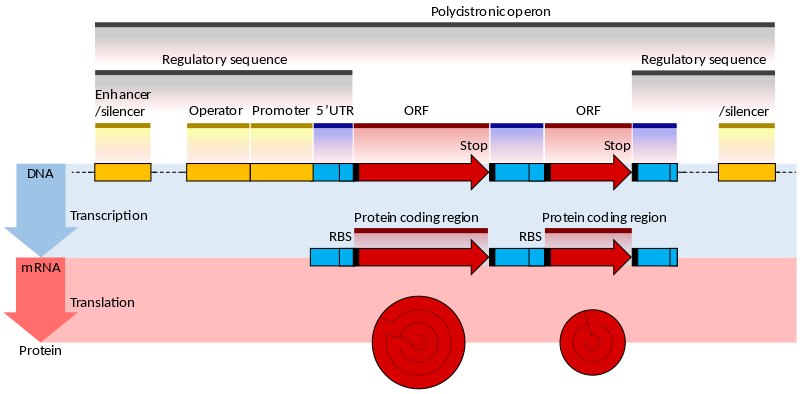 |
| From Wikipedia |
The genes of prokaryotes have well characterized promoter sequences containing known elements, such as the Pribnow box and transcription factor binding sites, that can be identified as markers for downstream genes. The coding sequence (CDS) is a long contiguous open reading frame (ORF), so detecting CDS together with the promoter is already a good indication of the presence of a real gene. Moreover, the bacterial genes are often contained in larger unit called operons.
| The eukaryotic gene |
|---|
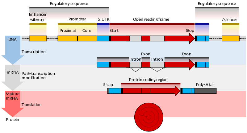 |
| From Wikipedia |
The genes of eukaryotes are more complex, since their promoters are more diverse and the CDS is broken into exons separated by noncoding introns. The programs designed for predicting eukaryotic genes search for additional signals such as:
- presence of CpG islands
- presence of binding sites for polyA tail
- different ORFs
- donor / acceptor splice sites
In most cases, programs like GLIMMER and GeneMark for prokaryotes, Augustus and Geneid for eukaryotes create a complex probabilistic model that can be pre-trained on a closest species to better achieve their aim.
The noncoding genes can be searched in a similar way using probabilistic models that join both information for the sequence and the RNA secondary structure; for example, the program Infernal that relies on the models stored in the Rfam database allows for detection of RNA gene families.
Empirical methods of genome annotation
Experimental evidences can be used to limit the number of false positives from the ab initio methods and to refine the predictions (for example improving the UTR boundaries).
They can also be used to add novel genes that are intrinsically difficult to find, such as the short genes, the long noncoding RNA, etc.
RNA sequences obtained by transcritome sequencing can be used to inform genome annotation by being mapped to the assembled genome. The main drawback of this approach is that in complex organisms only a fraction of genes is expressed at certain time and their expression is also tissue specific.
The genomes stored in public repositories also contain annotations which you can see in the GenBank format under the tab FEATURES. This annotation can be also downloaded in the GFF3 format, using the top right tab Send to -> Complete Record / Choose Destination: File / Format GFF3.
##sequence-region MN908947.3 1 29903
##species https://www.ncbi.nlm.nih.gov/Taxonomy/Browser/wwwtax.cgi?id=2697049
MN908947.3	Genbank	region	1	29903	.	+	.	ID=MN908947.3:1..29903;Dbxref=taxon:2697049;collection-date=Dec-2019;country=China;gbkey=Src;genome=genomic;isolate=Wuhan-Hu-1;mol_type=genomic RNA;nat-host=Homo sapiens
MN908947.3	Genbank	five_prime_UTR	1	265	.	+	.	ID=id-MN908947.3:1..265;gbkey=5'UTR
MN908947.3	Genbank	gene	266	21555	.	+	.	ID=gene-orf1ab;Name=orf1ab;gbkey=Gene;gene=orf1ab;gene_biotype=protein_coding
MN908947.3	Genbank	CDS	266	13468	.	+	0	ID=cds-QHD43415.1;Parent=gene-orf1ab;Dbxref=NCBI_GP:QHD43415.1;Name=QHD43415.1;Note=translated by -1 ribosomal frameshift;exception=ribosomal slippage;gbkey=CDS;gene=orf1ab;product=orf1ab polyprotein;protein_id=QHD43415.1
MN908947.3	Genbank	CDS	13468	21555	.	+	0	ID=cds-QHD43415.1;Parent=gene-orf1ab;Dbxref=NCBI_GP:QHD43415.1;Name=QHD43415.1;Note=translated by -1 ribosomal frameshift;exception=ribosomal slippage;gbkey=CDS;gene=orf1ab;product=orf1ab polyprotein;protein_id=QHD43415.1
MN908947.3	Genbank	gene	21563	25384	.	+	.	ID=gene-S;Name=S;gbkey=Gene;gene=S;gene_biotype=protein_coding
MN908947.3	Genbank	CDS	21563	25384	.	+	0	ID=cds-QHD43416.1;Parent=gene-S;Dbxref=NCBI_GP:QHD43416.1;Name=QHD43416.1;Note=structural protein;gbkey=CDS;gene=S;product=surface glycoprotein;protein_id=QHD43416.1
MN908947.3	Genbank	gene	25393	26220	.	+	.	ID=gene-ORF3a;Name=ORF3a;gbkey=Gene;gene=ORF3a;gene_biotype=protein_coding
MN908947.3	Genbank	CDS	25393	26220	.	+	0	ID=cds-QHD43417.1;Parent=gene-ORF3a;Dbxref=NCBI_GP:QHD43417.1;Name=QHD43417.1;gbkey=CDS;gene=ORF3a;product=ORF3a protein;protein_id=QHD43417.1
MN908947.3	Genbank	gene	26245	26472	.	+	.	ID=gene-E;Name=E;gbkey=Gene;gene=E;gene_biotype=protein_coding
MN908947.3	Genbank	CDS	26245	26472	.	+	0	ID=cds-QHD43418.1;Parent=gene-E;Dbxref=NCBI_GP:QHD43418.1;Name=QHD43418.1;Note=structural protein%3B E protein;gbkey=CDS;gene=E;product=envelope protein;protein_id=QHD43418.1
MN908947.3	Genbank	gene	26523	27191	.	+	.	ID=gene-M;Name=M;gbkey=Gene;gene=M;gene_biotype=protein_coding
MN908947.3	Genbank	CDS	26523	27191	.	+	0	ID=cds-QHD43419.1;Parent=gene-M;Dbxref=NCBI_GP:QHD43419.1;Name=QHD43419.1;Note=structural protein;gbkey=CDS;gene=M;product=membrane glycoprotein;protein_id=QHD43419.1
MN908947.3	Genbank	gene	27202	27387	.	+	.	ID=gene-ORF6;Name=ORF6;gbkey=Gene;gene=ORF6;gene_biotype=protein_coding
MN908947.3	Genbank	CDS	27202	27387	.	+	0	ID=cds-QHD43420.1;Parent=gene-ORF6;Dbxref=NCBI_GP:QHD43420.1;Name=QHD43420.1;gbkey=CDS;gene=ORF6;product=ORF6 protein;protein_id=QHD43420.1
MN908947.3	Genbank	gene	27394	27759	.	+	.	ID=gene-ORF7a;Name=ORF7a;gbkey=Gene;gene=ORF7a;gene_biotype=protein_coding
MN908947.3	Genbank	CDS	27394	27759	.	+	0	ID=cds-QHD43421.1;Parent=gene-ORF7a;Dbxref=NCBI_GP:QHD43421.1;Name=QHD43421.1;gbkey=CDS;gene=ORF7a;product=ORF7a protein;protein_id=QHD43421.1
MN908947.3	Genbank	gene	27894	28259	.	+	.	ID=gene-ORF8;Name=ORF8;gbkey=Gene;gene=ORF8;gene_biotype=protein_coding
MN908947.3	Genbank	CDS	27894	28259	.	+	0	ID=cds-QHD43422.1;Parent=gene-ORF8;Dbxref=NCBI_GP:QHD43422.1;Name=QHD43422.1;gbkey=CDS;gene=ORF8;product=ORF8 protein;protein_id=QHD43422.1
MN908947.3	Genbank	gene	28274	29533	.	+	.	ID=gene-N;Name=N;gbkey=Gene;gene=N;gene_biotype=protein_coding
MN908947.3	Genbank	CDS	28274	29533	.	+	0	ID=cds-QHD43423.2;Parent=gene-N;Dbxref=NCBI_GP:QHD43423.2;Name=QHD43423.2;Note=structural protein;gbkey=CDS;gene=N;product=nucleocapsid phosphoprotein;protein_id=QHD43423.2
MN908947.3	Genbank	gene	29558	29674	.	+	.	ID=gene-ORF10;Name=ORF10;gbkey=Gene;gene=ORF10;gene_biotype=protein_coding
MN908947.3	Genbank	CDS	29558	29674	.	+	0	ID=cds-QHI42199.1;Parent=gene-ORF10;Dbxref=NCBI_GP:QHI42199.1;Name=QHI42199.1;gbkey=CDS;gene=ORF10;product=ORF10 protein;protein_id=QHI42199.1
MN908947.3	Genbank	three_prime_UTR	29675	29903	.	+	.	ID=id-MN908947.3:29675..29903;gbkey=3'UTR
The General Feature Format (GFF) format consists of one line per feature, each containing 9 columns of data, plus optional track definition lines indicated by the first character ”#”.
| Column number | Column name | Details |
|---|---|---|
| 1 | seqname | name of the chromosome or scaffold; chromosome names can be given with or without the ‘chr’ prefix. |
| 2 | source | name of the program that generated this feature, or the data source (database or project name) |
| 3 | feature | feature type name, e.g. Gene, Variation, Similarity |
| 4 | start | Start position of the feature, with sequence numbering starting at 1. |
| 5 | end | End position of the feature, with sequence numbering starting at 1. |
| 6 | score | A floating point value. |
| 7 | strand | defined as + (forward) or - (reverse). |
| 8 | frame | One of ‘0’, ‘1’ or ‘2’. ‘0’ indicates that the first base of the feature is the first base of a codon, ‘1’ that the second base is the first base of a codon, and so on.. |
| 9 | attribute | A semicolon-separated list of tag-value pairs, providing additional information about each feature. |
Here you can see the reference sequences of the human genome. We can open the Y chromosome and get the graphical view clicking on Graphics.
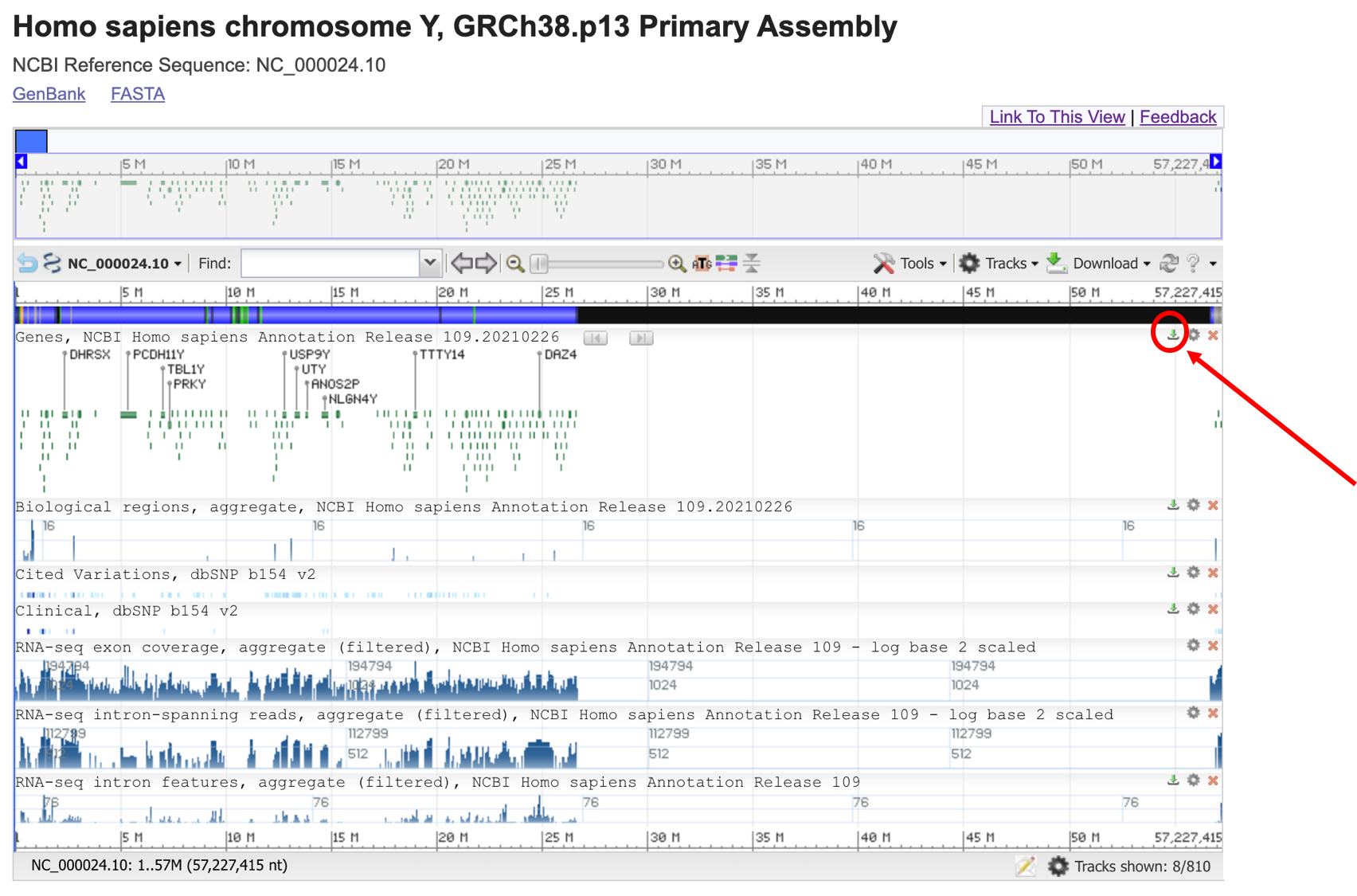
Here you can select the range that you prefer in the chromosome for zooming or highlighting. Then you can export the annotation information by clicking on the small green arrow icon indicated by the red circle.
Exercise: For the NCBI genome with Accession number MT020880 download the annotation file, open it in a text editor and answer the following questions:
- Can you guess the genome size?
- How many genes were annotated for this genome?
- Which genome position encode for the nucleocapsid phosphoprotein, which is the corresponding gene identifier?
- How many genes are on the strand “minus”?
- Moving again to the human Y chromosome, can you extract the genes between the position 5,000,000 and 6,000,000? How many genes and pseudogenes do you get? On which strand are they? How many alternative transcripts are found for the first gene?
Public resources hosting genomes
Currently there are different databases that host genomic sequences with their annotations:
- ENSEMBL genomes from European Bioinformatics Institute and the Wellcome Trust Sanger Institute.
- GENCODE from a consortium annotating Mouse and Human genomes.
- UCSC genome browser from the University of California, Santa Cruz (UCSC).
- NCBI genomes from National Center for Biotechnology Information, USA.
- GOLD from the DOE Joint Genome Institute.
Some of these online resources also allow displaying information about the genome in a graphical way in the web browser (aka Genome Browser).