Protein-DNA interactions
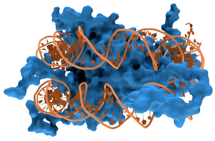
Different class of proteins are known to bind nucleic acids thanks to some domains that have affinities for single or double stranded DNA or RNA. The proteins that bind DNA can be classified into:
- Non-specific DNA-binding proteins, such as histones, polymerases and helicases.
- Specific DNA-binding proteins, such as transcription factors.
Specific DNA sequences bound by a protein can be identified using the following experiments:
- EMSA (electrophoretic mobility shift assay, or gel shift assay). It is a common affinity electrophores technique used to study protein–DNA or protein–RNA interactions. This procedure can determine if a protein or mixture of proteins is capable of binding to a given DNA or RNA sequence, and can sometimes indicate if more than one protein molecule is involved in the binding complex.
- DNA pull-down assay. Pull-down assays are used to selectively extract a protein–DNA complex from a sample. Typically, the pull-down assay uses a DNA probe labeled with a high affinity tag, such as biotin, which allows the probe to be recovered or immobilized. A biotinylated DNA probe can be complexed with a protein from a cell lysate in a reaction similar to that used in the EMSA and then used to purify the complex using agarose or magnetic beads. The proteins are then eluted from the DNA and detected by western blot or identified by mass spectrometry.
- SELEX. It is stands for Systematic Evolution of Ligands by EXponential Enrichment. SELEX is an experimental procedure that involves the progressive selection, from a large combinatorial double-stranded oligonucleotide library, of proteins with variable DNA-binding affinities and specificities by repeated rounds of partition and amplification.
- ChIP-on-chip. The complex protein DNA is fixed using crosslinking and then pulled down using an antibody specific for the protein. The crosslink is then reverted and the bound sequences hybridized on a microarray chip to discover the bound genes.
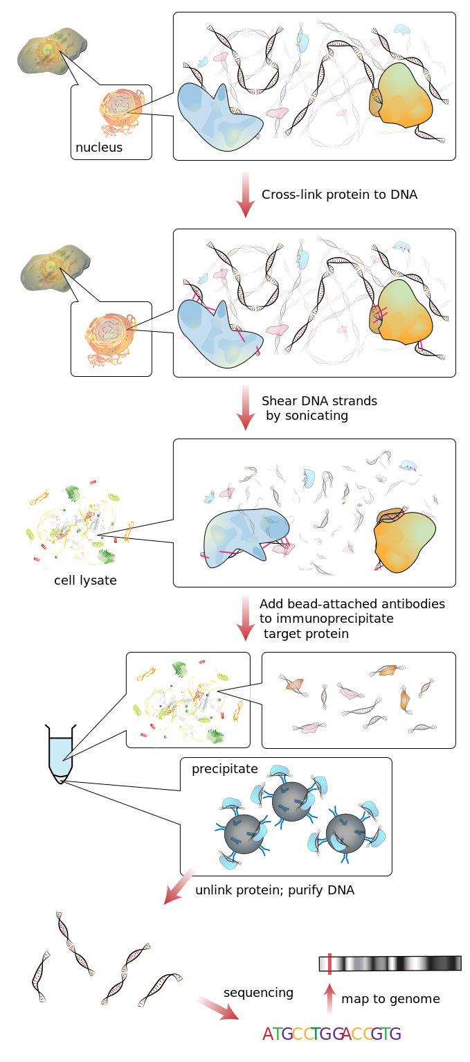
- ChIP-Seq. Similar to the ChIP-on-chip but it is a direct sequencing of the DNA captured by the immunoprecipitated protein.
ChIP-Seq workflow
Frow wikipedia:
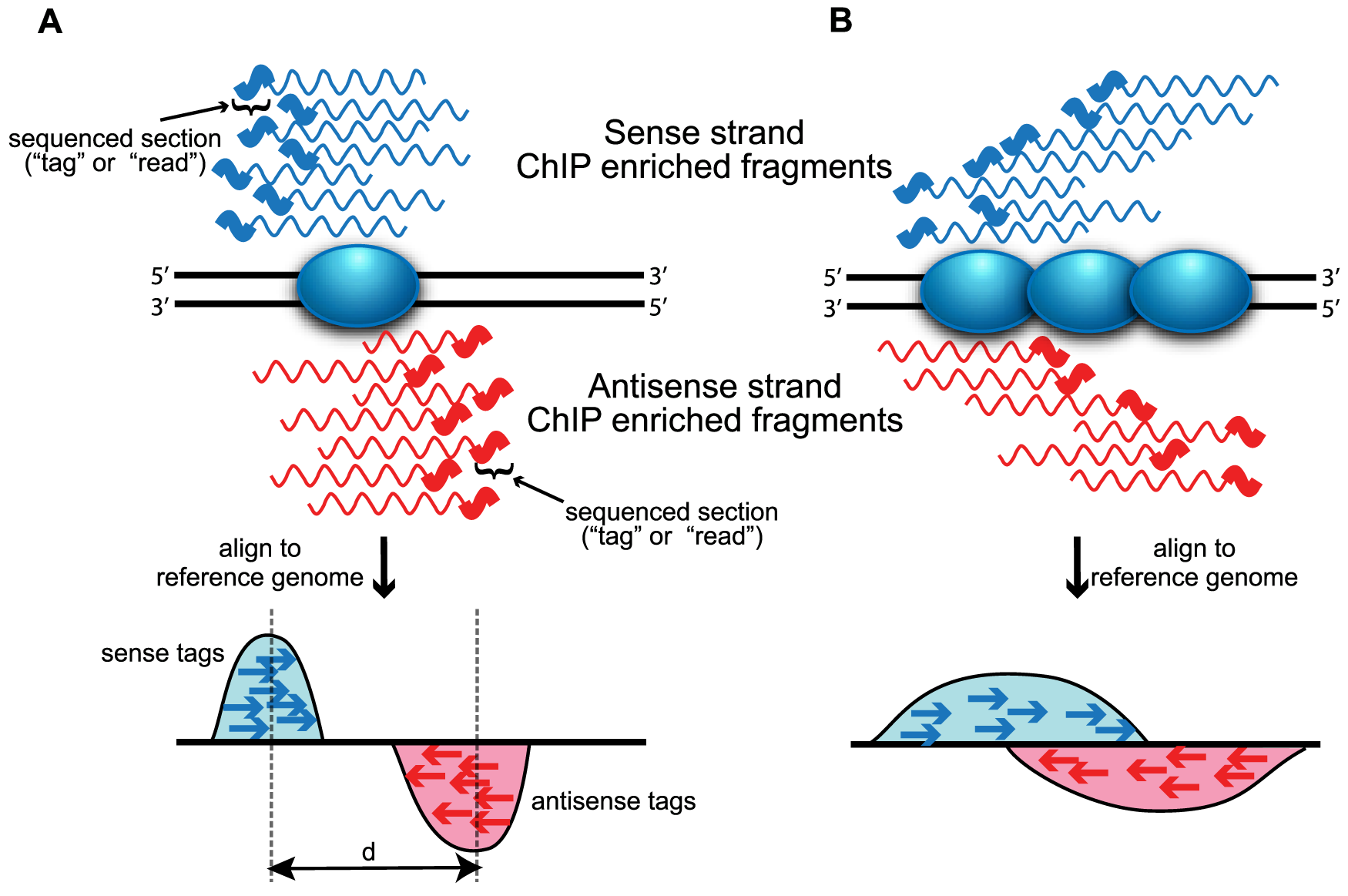
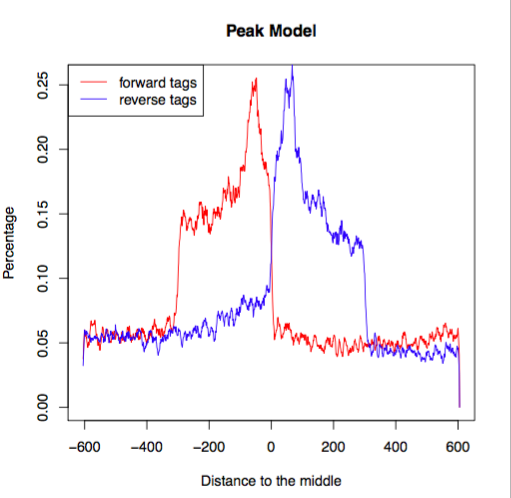
Peak calling
 |
| From: Evaluation of Algorithm Performance in ChIP-Seq Peak Detection, Elizabeth G et al. PLoS One 2010 |
ChIP-Seq data repositories
Raw sequencing data and results from ChIPseq experiments generally have to be uploaded to public repositories for supporting scientific publications. The two mostly used repositories:
- Gene Expression Omnibus (GEO) from NCBI
- ArrayExpress from EMBL/EBI
Until 2016 these two databases were mirroring each other.
GEO
We will focus now on GEO, and this “Series of experiments “GSE41589” in particular.
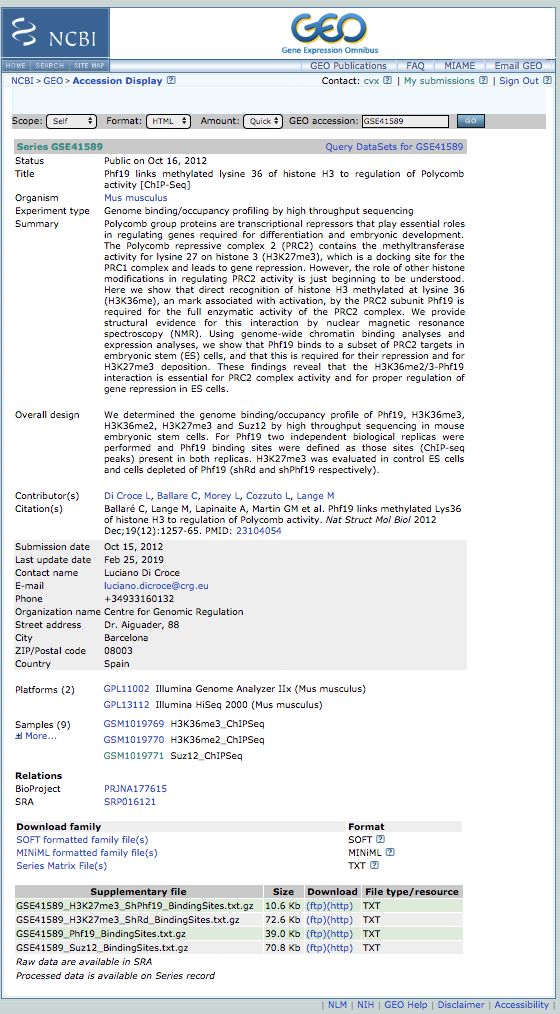
As you can see, GEO provides information about the study and experiment including the overall design, the sequencing platform used (indicated by identifiers strating with GPL), samples (indicated with the prefix GSM), the BioProject identifier PRJNA177615 and the SRA identifier SRP016121. Finally a list of result files. An important file containing all the metadata about a GEO dataset is given as SOFT formatted family file(s). If you download it you can know also some hidden information like the version of the genome used.
- Sequence Read Archive (SRA) collects all the raw sequencing data together with information about the sequencing method.
- BioProject is a collection of biological data related to a single initiative, originating from a single organization or from a consortium. A BioProject record provides users a single place to find links to the diverse data types generated for that project.
The analysis of ChIP-Seq data produces a list of genomic positions (aka, peaks) with some probability/score to be bound to a protein of interest. The higher the number of reads found in that genomic position, together with the a low number of mapped tags in the control, the higher the probability that the binding event is not a false positive one.
Let’s download such a list of the Suz12 protein binding regions which is provided in the file GSE41589_Suz12_BindingSites.txt.gz. This list of peaks is represented in a tabular format called BED format, which is a standard format for the results of any ChIP-Seq data analysis. The BED file has one line per feature (in this case, a peak, or the genome region to which a protein binds), each containing between 3 and 12 columns of data.
The typical 6-field BED format:
| chrom | chromStart | chromEnd | name | score | strand |
|---|---|---|---|---|---|
| chr7 | 127471196 | 127472363 | Pos1 | 0 | + |
| chr7 | 127472363 | 127473530 | Pos2 | 0 | + |
| chr7 | 127473530 | 127474697 | Pos3 | 0 | + |
| chr7 | 127474697 | 127475864 | Pos4 | 0 | + |
Additionally you may have up to another 6 fields:
| thickStart | thickEnd | itemRgb | blockCount | blockSizes | blockStarts |
|---|---|---|---|---|---|
| 127471196 | 127472363 | 255,0,0 | 0 | 0 | 0 |
| 127472363 | 127473530 | 255,0,0 | 0 | 0 | 0 |
| 127473530 | 127474697 | 255,0,0 | 0 | 0 | 0 |
| 127474697 | 127475864 | 255,0,0 | 0 | 0 | 0 |
Exercise:
1)
- Which samples correspond to the ChIP-seq experiment of DNA binding of the Suz12 protein? Remember that we need two samples for doing this kind of experiment.
- How many regions of Suz12 binding were identified on chromosome Y?
- What is the distance between the first and the last peak on chromosome Y?
- How many sequences platforms have been used?
- Can you guess why some of them are named (Hi)?
- Why do we have two controls?
2)
- Let’s move to UCSC genome browser. Load the hg38 genome and try to load the peaks for Suz12 going in ENCODE REGULATION and looking inside TF clusters. Once loaded check the presence of a peak at the 5’ of the Suz12 gene itself. (If you need help you can read below).
- Now move to the mouse genome version mm9 and add the peak data obtained by the GEO entry in the UCSC genome browser as custom track. Look again at Suz12 and its promoter region. Do you find a similar peak than in human? (If you need help you can read below)
ChIP-Seq experiments in the UCSC Genome Browser
You already became familiar with UCSC Genome Browser in the session Genome sequences and annotations.
Searching for known experiments
Open the UCSC genome browser, select the latest assembly of the human genome, hg38, and click “GO”.
Scroll down to the tracks in the section REGULATION.
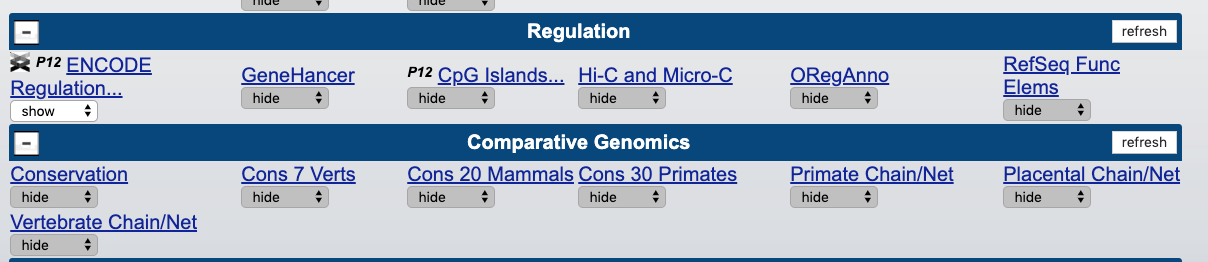
And click on the ENCODE link that will bring us at this page:
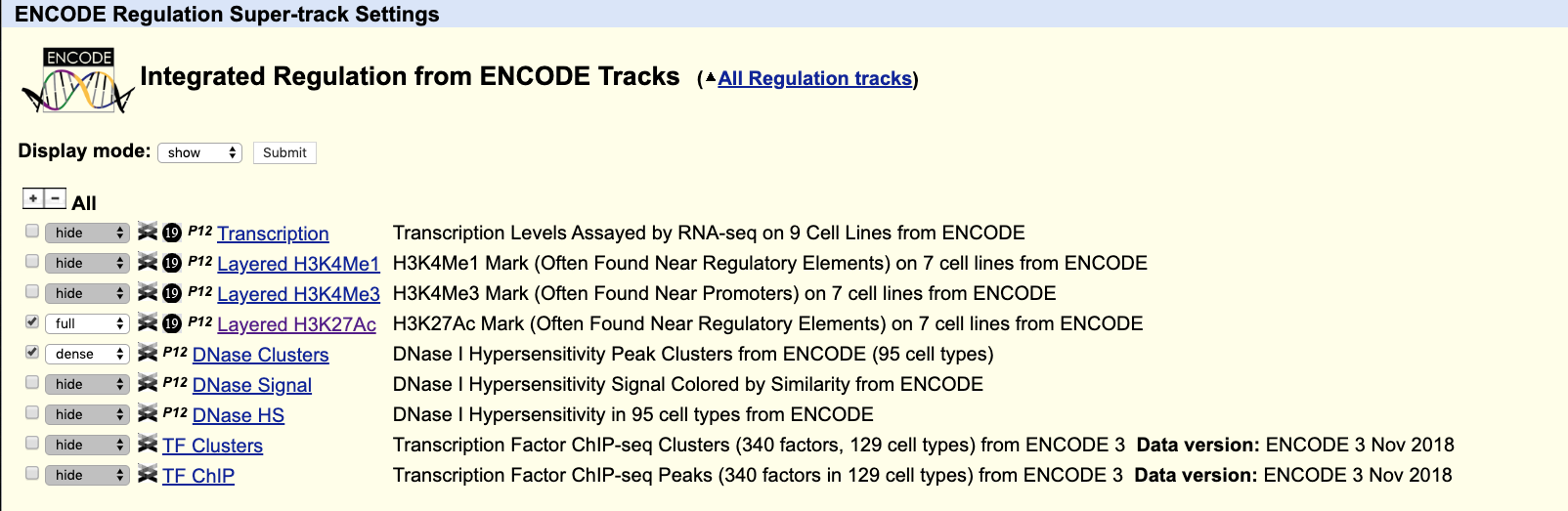
We can select either clusters or peak. The former will contain information about which cell line the peak is expressed while the second are available only for a given cell line (you have to select a cell line too).
Let’s click on the link “TF clusters”. On the top of the newly appeared page select “Full” for Display Mode and Filter by factor selecting Suz12 in the pulled down list. Click Submit on top of the page to return to the Browser.
Now let’s serach for the Suz12 gene to investigate if it binds to its own promoter. You can see the black box at the position chr17:31916990-31917580. The peak lies in the middle between TSS of the Suz12 gene going in 5’-3’ of one strand and TSS of the UTP6 gene on the other DNA strand; this is known as a bidirectional promoter. Clicking on the peak gives us information about the experiment and peak itself.
| signal | abr | cellType | factor | experiment | lab | more info | |
|---|---|---|---|---|---|---|---|
| 1 | 938.00 | G | GM12878 | SUZ12 | ENCSR091BOQ | bernstein | ENCFF547FUI |
Visualizing your own BED file of ChIP-seq peaks
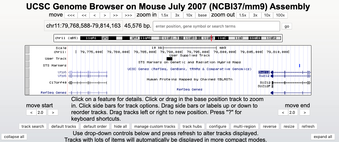
You can also add your own data to be visualized in the Genome Browser. Let’s move to the mouse genome (version mm9). We can upload the peak list we downloaded previously (the file GSE41589_Suz12_BindingSites.txt.gz) clicking on ADD CUSTOM TRACKS. Upload this file via Upload -> Choose file -> submit. Then, on a new page view in: -> Genome Browser -> go.
NOTE: We recommend always using compressed file for uploading since it will speed up the whole operation and reduce the risk of server time out.
We can search again for Suz12, zoom out to see black boxes on User Track on the top of other tracks. We can see that this peak between two genes is a conserved feature and we got it in our experiment similarly to the ENCODE experiment we visualized before.