Hands-on: Reference genome/transcriptome and annotation

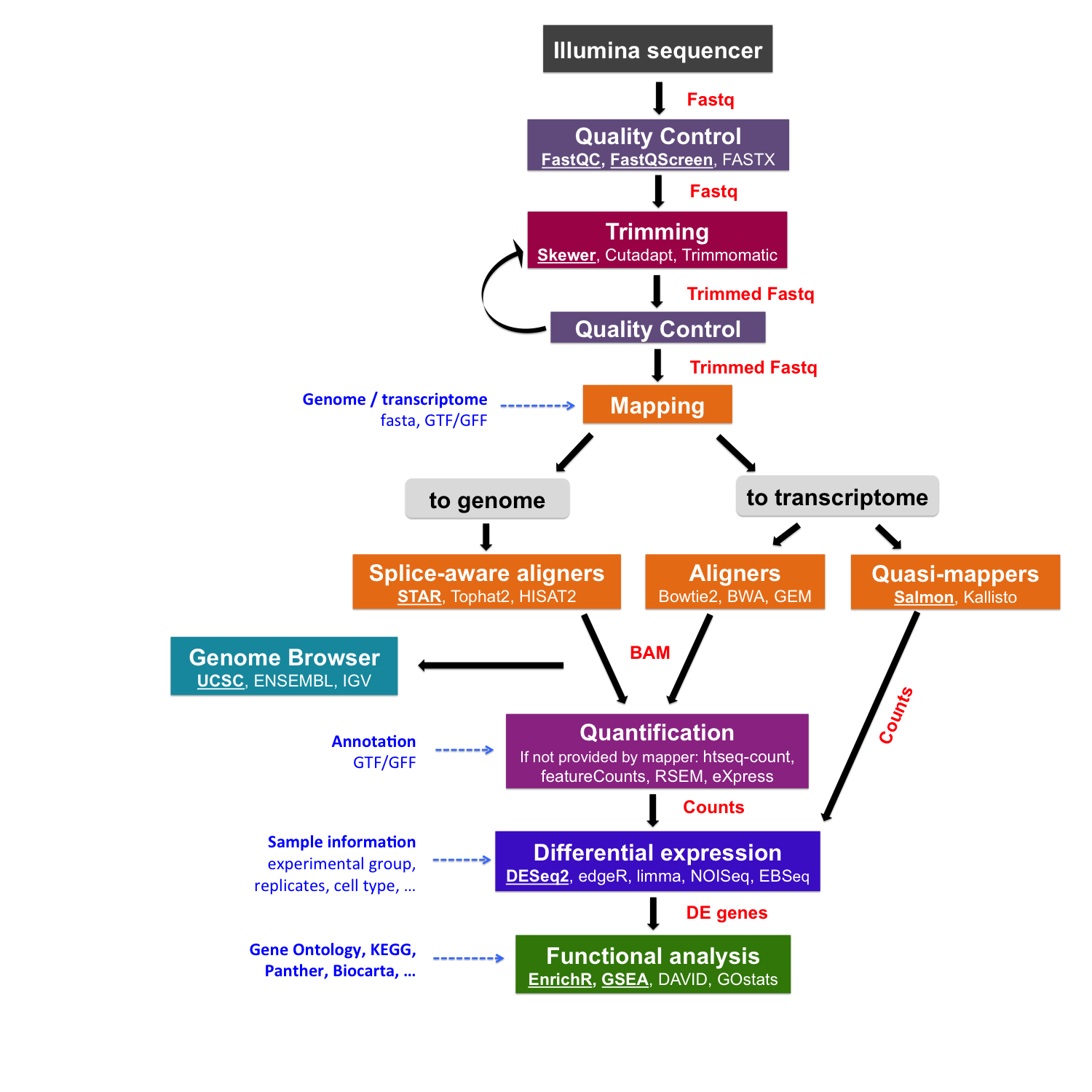
After sequencing, reads are pre-processed and quality-checked. The next step is to map them to a reference. This raises two key questions: “What references are available?” and “Which one should I use?”

Reference sequences

Before proceeding, we need to retrieve a reference genome or transcriptome from a public database, along with its annotation:

• A FASTA file contains the actual genome/transcriptome sequence.

• A GTF/GFF file contains the corresponding annotation.

Public resources on genome/transcriptome sequences and annotations

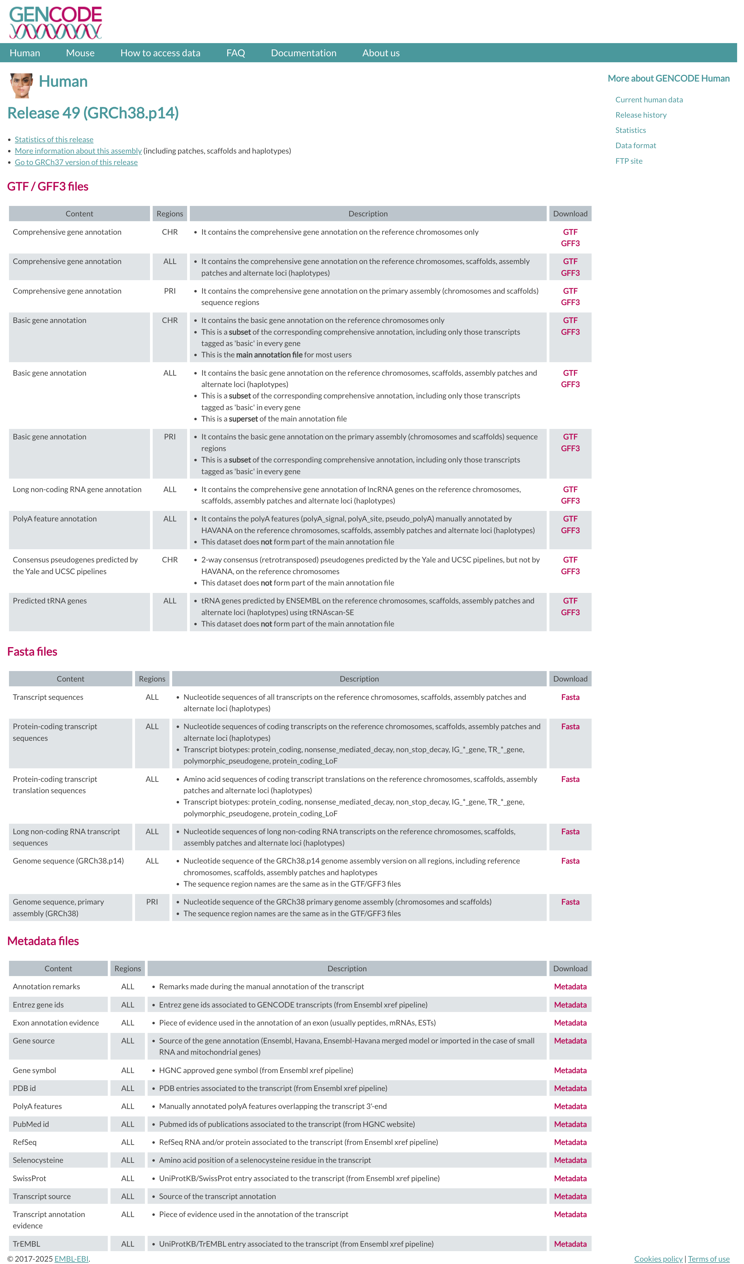
• GENCODE contains an accurate annotation of the human and mouse genes derived either using manual curation, computational analysis or targeted experimental approaches. GENCODE also contains information on functional elements, such as protein-coding loci with alternative splicing variants, non-coding loci, and pseudogenes.

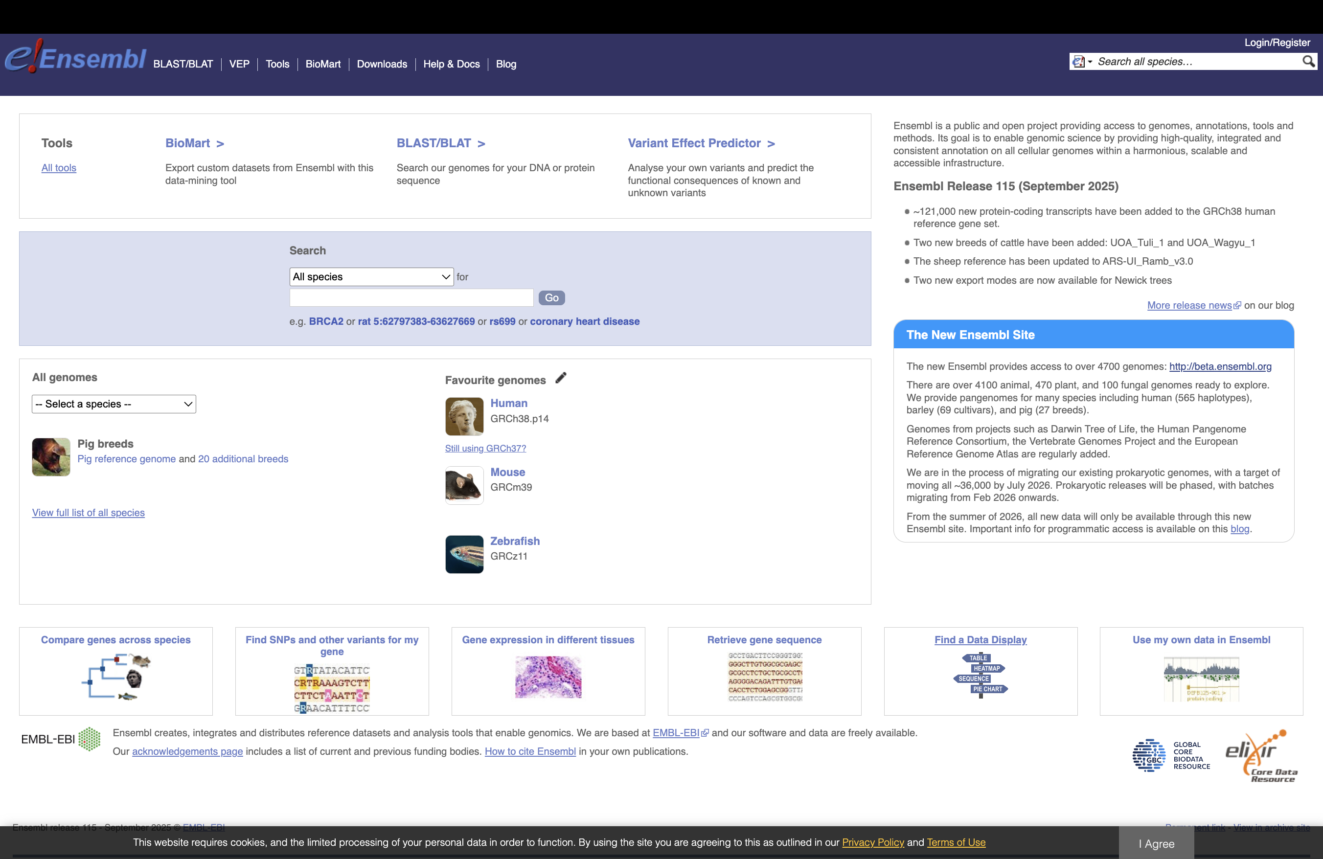
• Ensembl contains both automatically generated and manually curated annotations. They host different genomes together with comparative genomics data and their variants. Ensembl genomes extends the genomic information across different taxonomic groups: bacteria, fungi, metazoa, plants, and protists. Ensembl also integrates a genome browser.

• UCSC Genome Browser hosts information about different genomes. It integrates the GENCODE and Ensembl information as additional tracks.

Where to find the files

GENCODE

The current version for Homo sapiens genome is release 49.
The files you would need are:

• FASTA file for the Genome sequence, primary assembly

• FASTA file corresponding to the transcripts

• GTF file of the Comprehensive gene annotation

You can retrieve them via command line typing:

# genome
wget ftp://ftp.ebi.ac.uk/pub/databases/gencode/Gencode_human/release_49/GRCh38.primary_assembly.genome.fa.gz

# transcriptome
wget ftp://ftp.ebi.ac.uk/pub/databases/gencode/Gencode_human/release_49/gencode.v49.transcripts.fa.gz

# annotation
wget ftp://ftp.ebi.ac.uk/pub/databases/gencode/Gencode_human/release_49/gencode.v49.annotation.gtf.gz

ENSEMBL

The current version of the Mus musculus genome in Ensembl is release 115

The files you would need are:

• FASTA file for the genome primary assembly

• FASTA file corresponding to the CDS regions / transcripts

• GTF file for the annotation

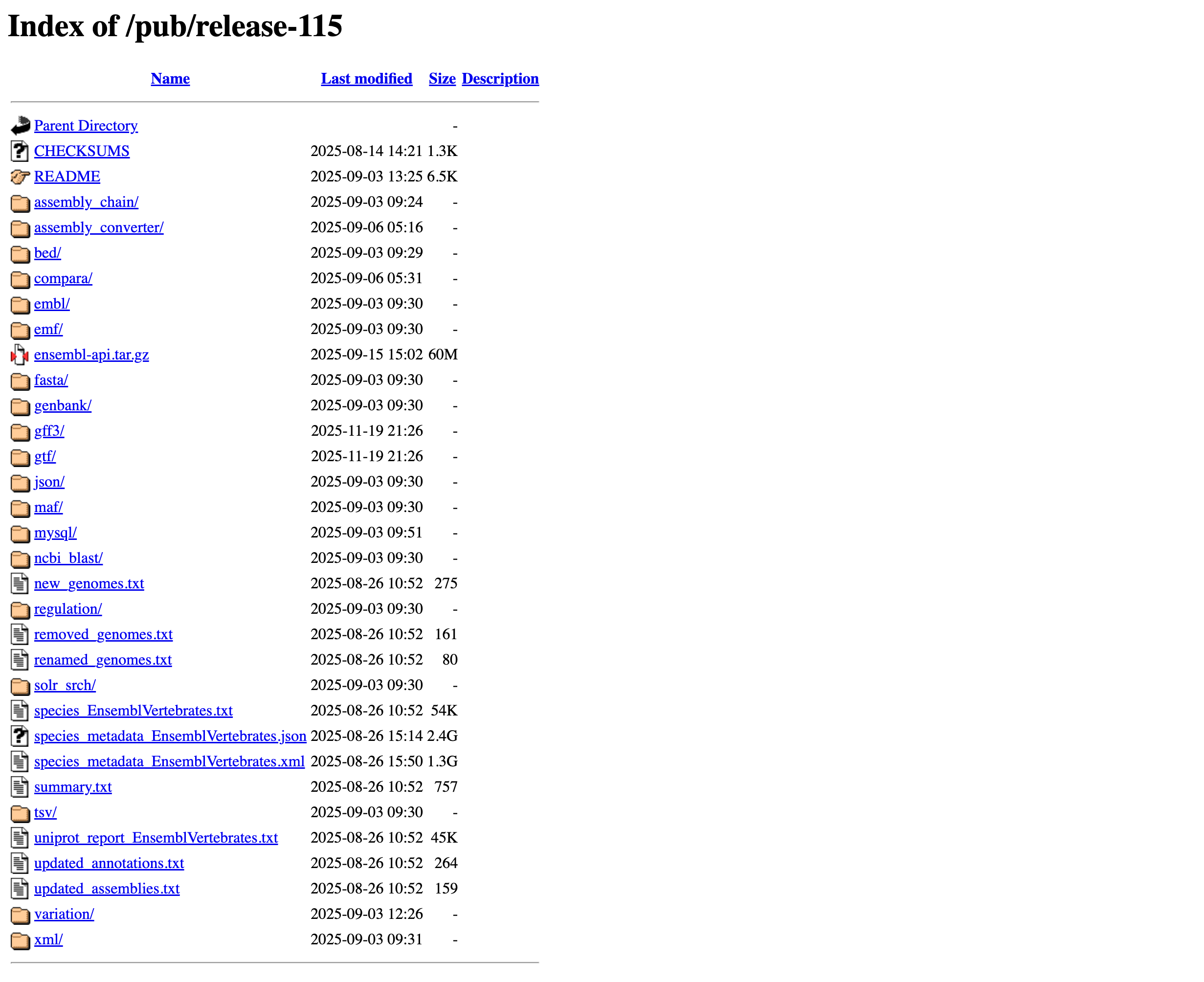
# genome
wget ftp://ftp.ensembl.org/pub/release-115/fasta/homo_sapiens/dna/Homo_sapiens.GRCh38.dna_rm.primary_assembly.fa.gz

# transcriptome
wget ftp://ftp.ensembl.org/pub/release-115/fasta/homo_sapiens/cds/Homo_sapiens.GRCh38.cds.all.fa.gz

# annotation
wget ftp://ftp.ensembl.org/pub/release-115/gtf/homo_sapiens/Homo_sapiens.GRCh38.115.chr.gtf.gz

Our data set

To speed up the mapping process, we retrieved a subset of the FASTA and GTF files that correspond only to chromosome 6 here: reference_chr6_Hsapiens.tar.gz

You can download them from:

# go to the appropriate folder
cd ~/rnaseq_course/reference_genome

# download reference files for chromosome 6
wget https://biocorecrg.github.io/RNAseq_coursesCRG_2026/latest/data/annotation/reference_chr6_Hsapiens.tar.gz

# extract archive
tar -xvzf reference_chr6_Hsapiens.tar.gz

# remove remaining .tar.gz archive
rm reference_chr6_Hsapiens.tar.gz

FASTA file

The genome is often stored as a FASTA file (.fa file): each header (that can be chromosomes, transcripts, proteins), starts with “>”:

zcat reference_chr6/Homo_sapiens.GRCh38.dna.chrom6.fa.gz | head -n 1

The size of the chromosome (in bp) is already reported in the header, but we can check it as follows:

zcat ~/rnaseq_course/reference_genome/reference_chr6/Homo_sapiens.GRCh38.dna.chrom6.fa.gz | grep -v ">" | tr -d '\n' | wc -m  

# 170805979

We can also check the transcriptome sequences.

zcat gencode.v49.transcripts.chr6.fa.gz| head -n 4
>ENST00000604449.1|ENSG00000271530.1|OTTHUMG00000184610.1|OTTHUMT00000468943.1|WBP1LP12-201|WBP1LP12|331|processed_pseudogene|
AGGATAAGGAAGCCTGTGTGTGTACCAACAATCAAAGCTACATCTGTGACACAACAGGACACTGCTATGGGCAGTCTCAGTGTTGTAACTACTACTATGAACATTGGTGGTTCTGGCTGGCATGGACCATCACCATCATCCTGAGCTGCTGCTGTGTCTGCCACCACAGCCAAGCCAGCCCTCAAGTCCAGCAGTAGCAACATGAAATCAACCTGACTGCCTATCCAGAAGCCCGCAATTACTCAGTGCTACCATTTTATTTCACCAAACTATTTATTACCTTCTTATGAGGAAGTGGTGAACTAACCTCCACCTGTTTCCCTCCCTGTCT
>ENST00000405102.1|ENSG00000220212.1|OTTHUMG00000014107.1|OTTHUMT00000039615.1|OR4F1P-201|OR4F1P|938|unprocessed_pseudogene|
ATGGATGGAGAGAATCACTCAGTGGTATCTGAGTTTTTGTTTCTGGGACTCACTCATTCATGGGAGATCCAGCTCCTCCTCCTAGTGTTTTCCTCTGTGCTCTATGTGGCAAGCATTACTGGAAACATCCTCATTGTATTTTCTGTGACCACTGACCCTCACTTACACTCCCCCATGTACTTTCTACTGGCCAGTCTCTCCTTCATTGACTTAGGAGCCTGCTCTGTCACTTCTCCCAAGATGATTTATGACCTGTTCAGAAAGCGCAAAGTCATCTCCTTTGGAGGCTGCATCGCTCAAATCTTCTTCATCCACGTCATTGGTGGTGTGGAGATGGTGCTGCTCATAGCCATGGCCTTTGACAGTTATGTGGCCCTATTAAGCCCCTCCACTATCTGACCATTATGAGCCCAAGAATGTGCCTTTCATTTCTGGCTGTTGCCTGGACCCTTGGTGTCAGTCACTCCCTGTTCCAACTGGCATTTCTTGTTAATTTACCCTTCTGTGGCCCTAATGTGTTGGACAGCTTCTACTGTGACCTTCCTCGGCTTCTCAGACTAGCCTGTACCGACACCTACAGATTGCAGTTCATGGTCACTGTTAACAGTGGGTTTATCTGTGTGGGTACTTTCTTCATACTTGTAATCTCCTACATCTTCATCCTGTTTACTGTTTGGAAACATTCCTCAGGTGGTTCATCCAAGGCCCTTTCCACTCTTTCAGCTCACAGCACAGCGGTCCTTTTGTTCTTTGGTCCACCCATGTTTGTGTATACATGGCCACACCCTAATTCACAGATGGACAAGTTTCTGGCTATTTTTGATGCAGTTCTCACTCCTTTTCTGAATCCAGTTGTCTATACATTCAGGAATAAGGAGATGAAGGCAGCAATAAAGAGAGTATGCAAACAGCTAGTGATTTACAAGAAGATCTCATAA

As you can see, this is a multi fasta file with several sequences, each one with its own header that contains:

Field	Value	Meaning
Ensembl Transcript ID	ENST00000405102.1	Transcript identifier from Ensembl. The .1 indicates the annotation version of the transcript.
Ensembl Gene ID	ENSG00000220212.1	Gene identifier in Ensembl associated with this transcript. .1 indicates the gene version.
HAVANA Gene ID	OTTHUMG00000014107.1	Gene identifier from the HAVANA manual annotation project
HAVANA Transcript ID	OTTHUMT00000039615.1	Transcript identifier from HAVANA
Transcript Name	OR4F1P-201	Name of the transcript isoform. 201 indicates the isoform number.
Gene Symbol	OR4F1P	Gene symbol (olfactory receptor family 4 member F1 pseudogene).
Transcript Length	938	Length of the transcript in base pairs (bp).
Gene Biotype	unprocessed_pseudogene	Gene type indicating a duplicated gene that lost protein-coding ability but retains intron–exon structure.

Exercise

• We can count how many transcripts we have in our fasta file by counting the character “>” that is in the header:

Solution

zcat gencode.v49.transcripts.chr6.fa.gz| grep ">" -c 
25648

• We can count the number of Gene Biotype by using a combination of linux commands such as grep, cut, sort, and uniq:

Solution

zcat gencode.v49.transcripts.chr6.fa.gz| grep ">" | cut -d "|" -f8|sort|uniq -c 
  11435 lncRNA
     67 miRNA
    105 misc_RNA
    971 nonsense_mediated_decay
      3 non_stop_decay
    581 processed_pseudogene
      7 processed_transcript
   9665 protein_coding
   1042 protein_coding_CDS_not_defined
      2 protein_coding_LoF
   1335 retained_intron
      1 rRNA
     26 rRNA_pseudogene
      1 scaRNA
     39 snoRNA
    107 snRNA
     34 TEC
     76 transcribed_processed_pseudogene
     11 transcribed_unitary_pseudogene
     63 transcribed_unprocessed_pseudogene
      3 unitary_pseudogene
     74 unprocessed_pseudogene

GTF file

The annotation is stored in General Transfer Format (GTF) format (which is an extension of the older GFF format): a tabular format with one line per genome feature, each one containing 9 columns of data. In general it has a header indicated by the first character “#” and one row per feature composed in 9 columns:

Column number	Column name	Details
1	seqname	name of the chromosome or scaffold; chromosome names can be given with or without the ‘chr’ prefix.
2	source	name of the program that generated this feature, or the data source (database or project name)
3	feature	feature type name, e.g. Gene, Variation, Similarity
4	start	Start position of the feature, with sequence numbering starting at 1.
5	end	End position of the feature, with sequence numbering starting at 1.
6	score	A floating point value.
7	strand	defined as + (forward) or - (reverse).
8	frame	One of ‘0’, ‘1’ or ‘2’. ‘0’ indicates that the first base of the feature is the first base of a codon, ‘1’ that the second base is the first base of a codon, and so on..
9	attribute	A semicolon-separated list of tag-value pairs, providing additional information about each feature.

zcat reference_chr6/Homo_sapiens.GRCh38.115.chr6.gtf.gz | head -n 10

Let’s check the 9th field:

zcat reference_chr6/Homo_sapiens.GRCh38.115.chr6.gtf.gz | cut -f9 | head

Let’s check how many genes are in the annotation file:

zcat reference_chr6/Homo_sapiens.GRCh38.115.chr6.gtf.gz | grep -v "#" | awk '$3=="gene"' | wc -l 

# 4230

You can also extract those genes and put them into a separate file:

zcat reference_chr6/Homo_sapiens.GRCh38.115.chr6.gtf.gz | grep -v "#" | awk '$3=="gene"' > genes.gtf

And get the final count of every feature:

zcat reference_chr6/Homo_sapiens.GRCh38.115.chr6.gtf.gz | grep -v "#" | cut -f3 | sort | uniq -c 

      1 
 101233 CDS
 172707 exon
  19185 five_prime_utr
   4230 gene
      3 Selenocysteine
  10180 start_codon
   9955 stop_codon
  16561 three_prime_utr
  25648 transcript

Exercise

Try to download the whole genome and annotation, and try to get the feature counts and count the number of Gene Biotype in the transcriptome.

Genome Browser

Read alignments (in BAM, CRAM, or BigWig formats) can be displayed in a genome browser, which is a program that allows users to browse, search, retrieve, and analyze genomic sequences and annotation data using a graphical interface.

There are two kinds of genome browsers:

• Web-based genome browsers:

  • UCSC Genome Broswer

  • Ensembl Genome Browser

  • NCBI Genome Data Viewer

• Desktop applications (some can also be used for generating a web-based genome browser):

  • JBrowse

  • GBrowse

  • IGV

Small-sized data can be directly uploaded to the genome browser, while large files are normally placed on a web server that is accessible to the browser. To explore BAM and CRAM files produced by the STAR mapper, we first need to sort and index the files.

UCSC Genome Browser

We uploaded the files for this project (chromosome 6 only) to:https://biocorecrg.github.io/RNAseq_coursesCRG_2026/latest/data/aln/index.html

Using the mouse’s right click, copy the URL address of one of the BAM files.

Now go to the UCSC genome browser website.

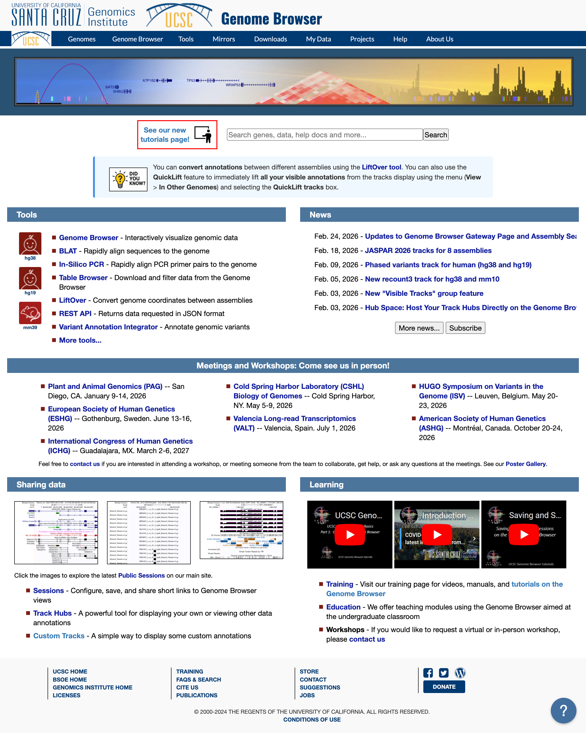
Choose human genome version hg38 (that corresponds to the ENSEMBL annotation we used). Click GO.

At the bottom of the image, click ADD CUSTOM TRACK

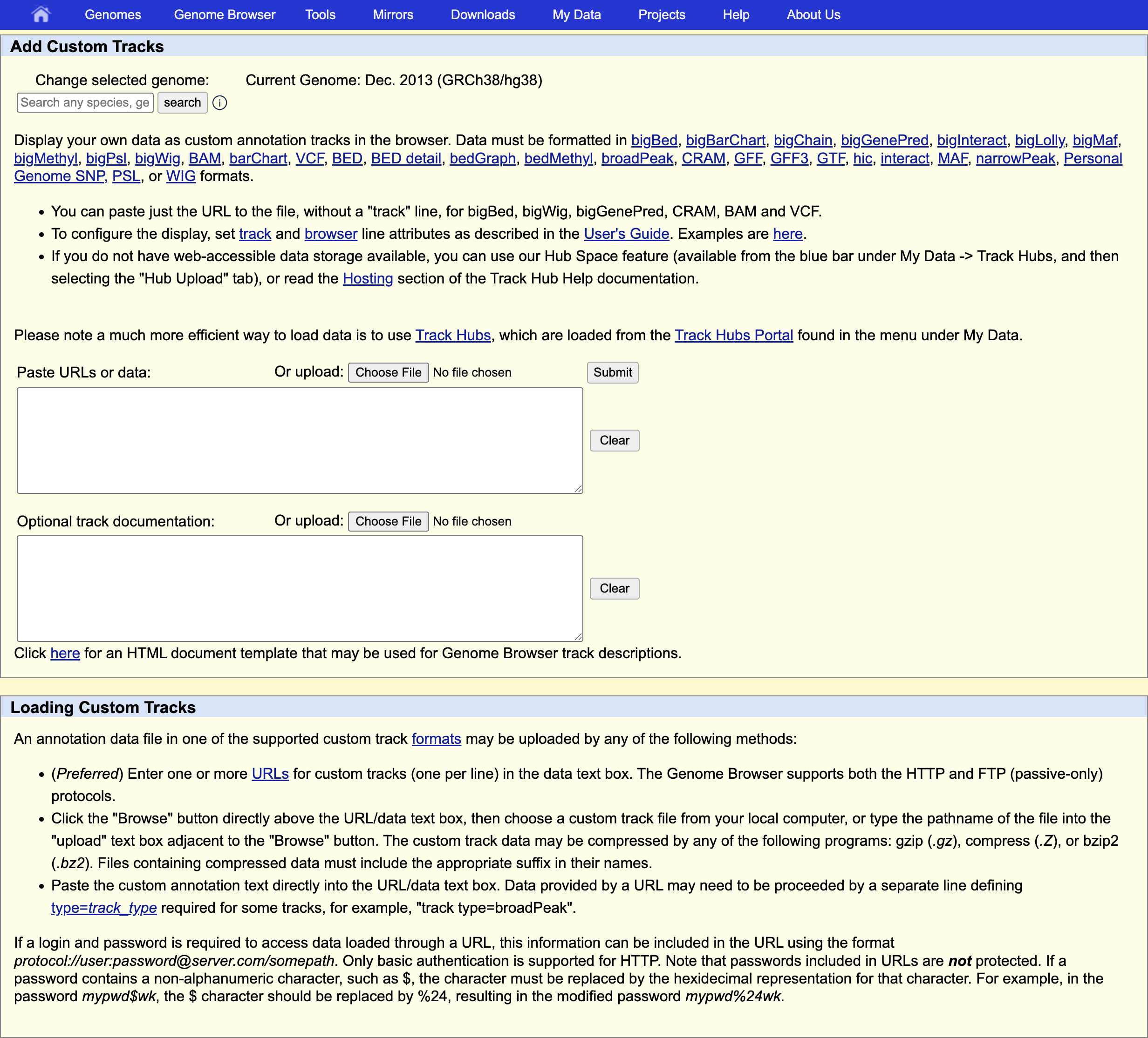
and provide information describing the data to be displayed:

• track type indicates the kind of file: bam (same is used for uploading .cram)

• name of the track

• bigDataUrl the URL where the BAM or CRAM file is located

track type=bam name="test" bigDataUrl=https://biocorecrg.github.io/RNAseq_coursesCRG_2026/latest/data/aln/SRR3091420_1_chr6Aligned.sortedByCoord.out.bam

Click “Submit”.

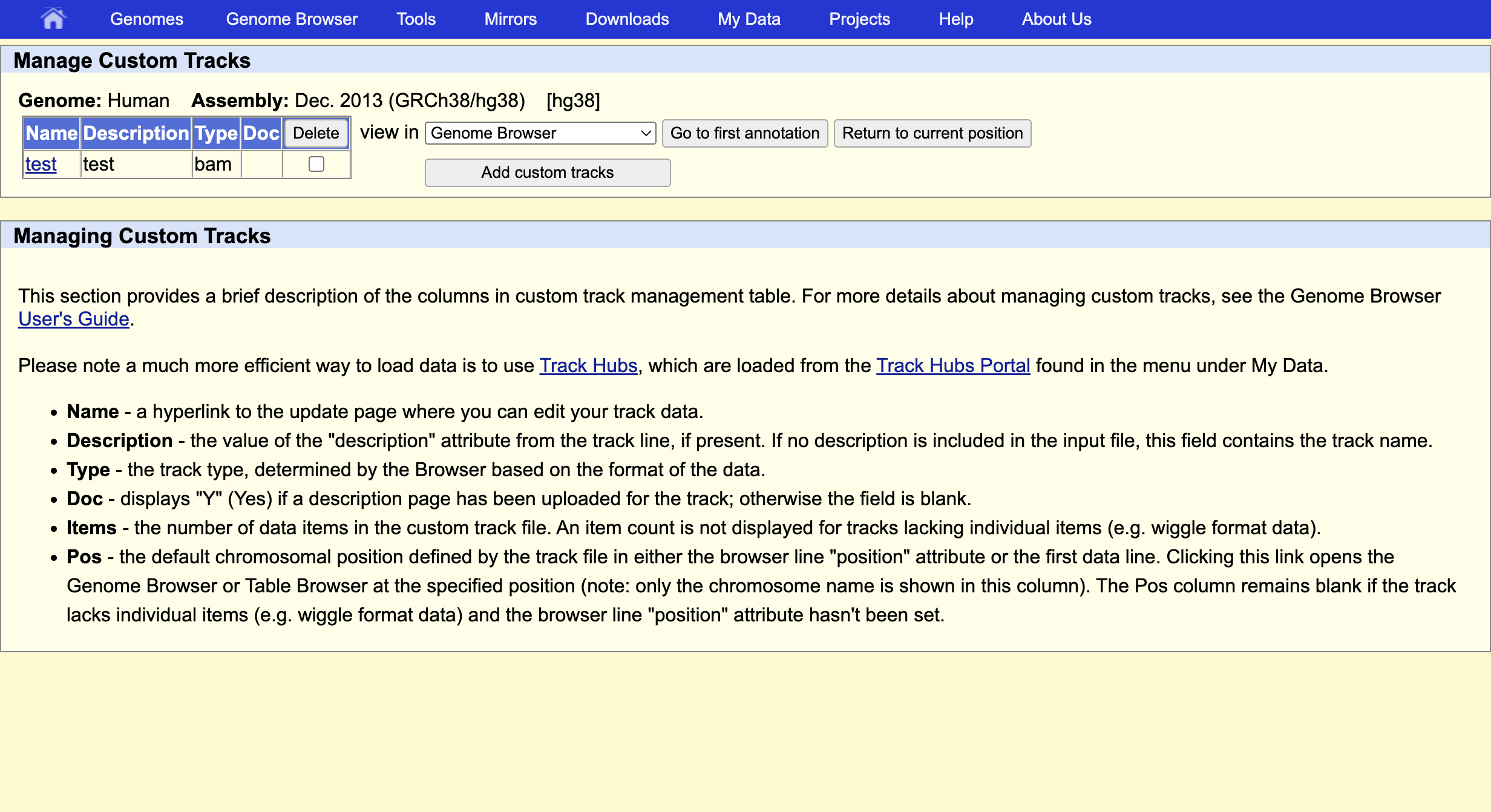
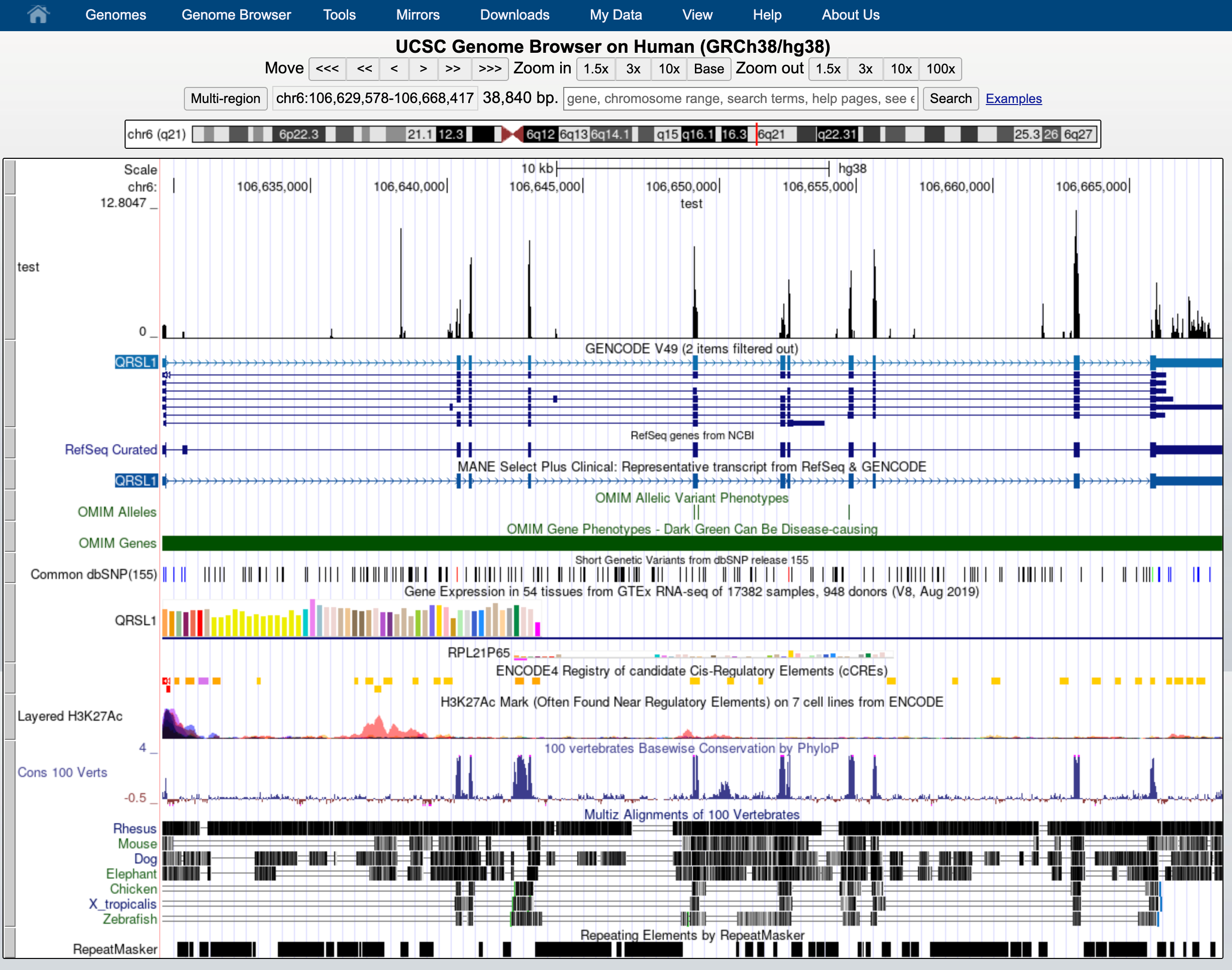
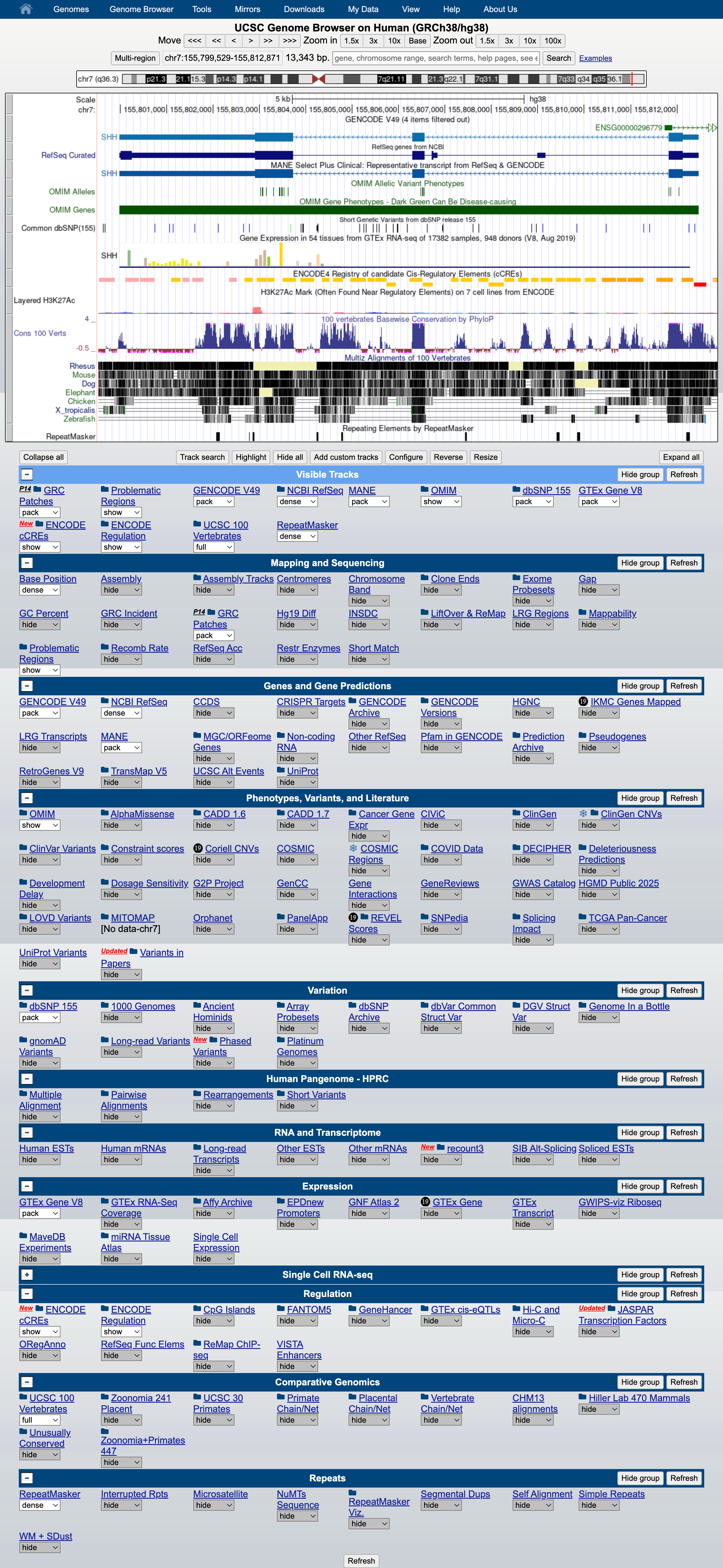
This indicates that everything went ok and we can now display the data. Since our data are restricted to chromosome 6 we have to display that chromosome. For example, let’s select the gene QRSL1 then go.

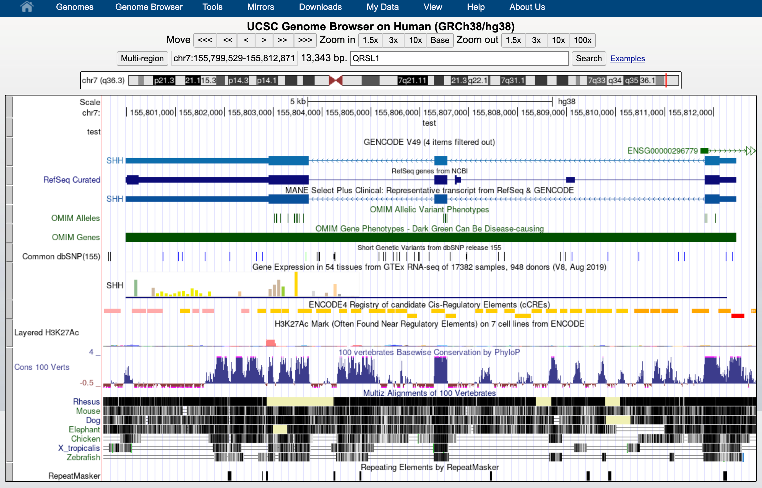
And we can display it.

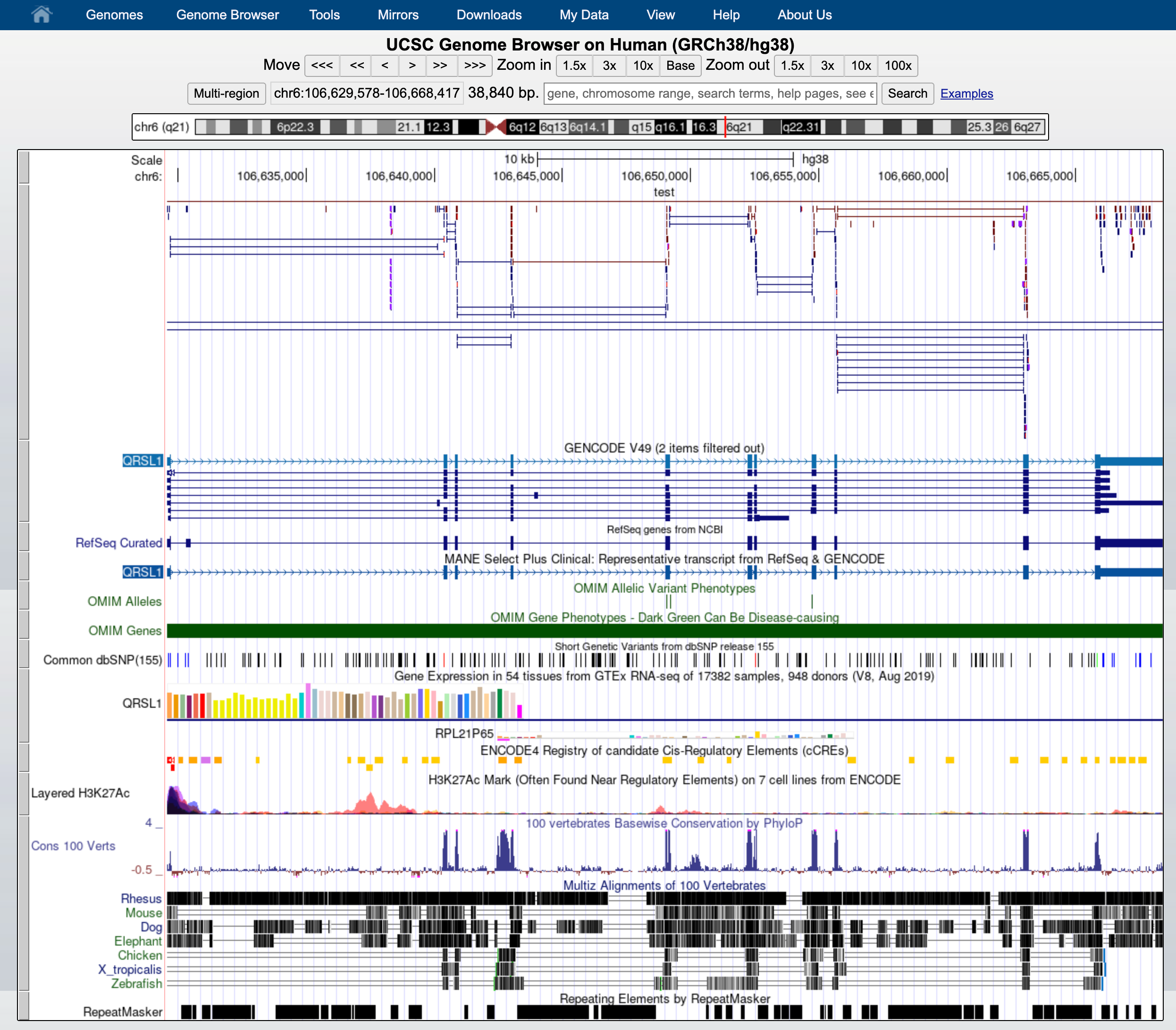
The default view can be changed by clicking on the grey bar on the left of the “My BAM” track. You can open a window with different settings; for example, you can change the Display mode to Squish.

This will change how data is displayed. We can now see single reads aligned to the forward and reverse DNA strands (blue is to +strand and red, to -strand). You can also see that many reads are broken; that is, they are mapped to splice junctions.

We can also display only the coverage by selecting in “My BAM Track Settings” Display data as a density graph and Display mode: full.

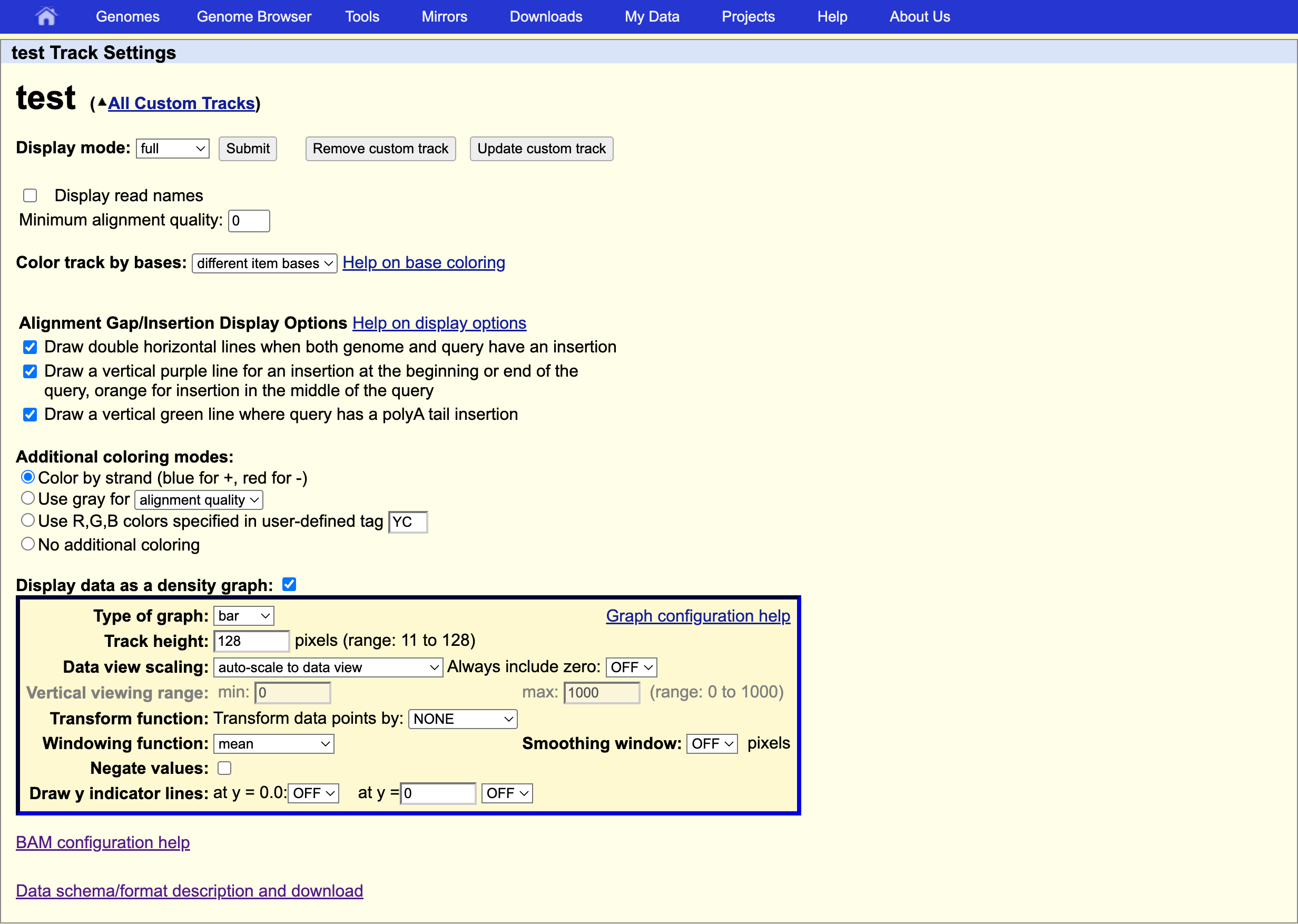
These expression signal plots can be helpful for comparing different samples (in this case, make sure to set comparable scales on the Y-axes).