Talk: Experimental design of RNA-seq experiment
Side note: scope of this course
This course focuses on bulk mRNA-seq experimental design and differential expression analysis. Many principles apply equally to total RNA-seq, small RNA-seq, scRNA-seq and long-read RNA-seq, but these technologies introduce additional considerations that are briefly noted throughout the material.
Reproducibility in RNA-seq
RNA-seq measures thousands of genes and relies on statistical models to detect differences between conditions.
Reproducibility is affected by:
sample size,
experimental variability,
technical bias.
Careful experimental design is required to:
reduce bias,
control variation,
estimate biological variability.
Important
Design determines whether RNA-seq results are interpretable.
Experimental design begins with the biological question
|
Figure is from https://galaxyproject.org/tutorials/rb_rnaseq/ |
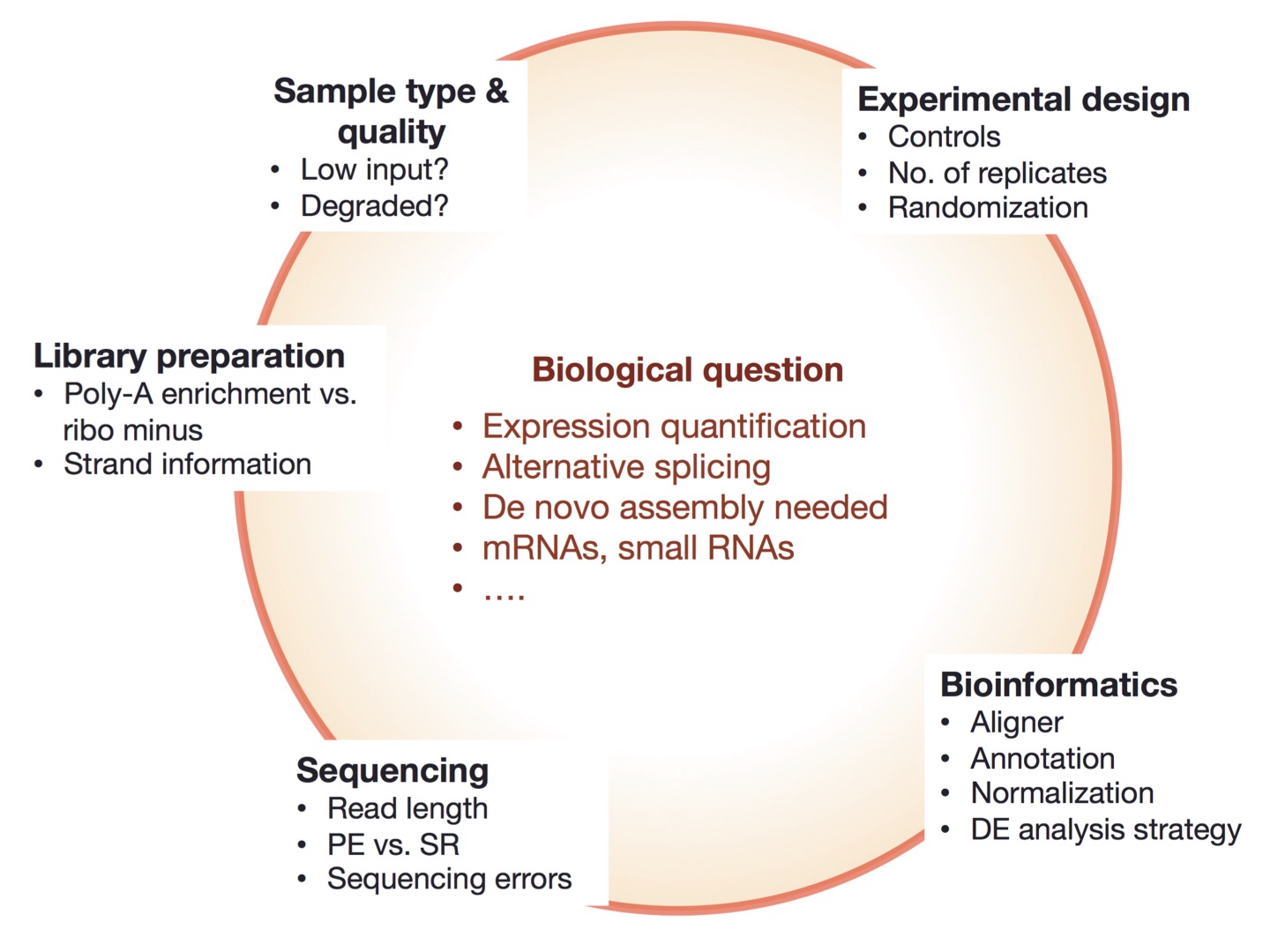
Think
biological question
→ experimental design
→ sample preparation
→ sequencing
→ analysis
Important
The biological question determines:
what to measure,
how to design the experiment,
and how to analyze the data.
Examples:
Which genes change expression between treated and control samples?
Do alternative isoforms differ between conditions?
Which cell types respond to treatment?
Core principles of RNA-seq experimental design
Replication → estimate biological variability
Randomization → avoid systematic bias
Blocking → control known sources of variation
In RNA-seq experiments:
replication → independent biological samples
randomization → distribute samples across batches and lanes
blocking → include batch in the model (design = ~ batch + condition)
Replication or Why independent samples are required
Replication allows estimation of biological variability, which determines whether observed differences are real.
Golden rule of replication
Replicates must be independent biological units, not repeated measurements of the same sample.
Experimental unit
The experimental unit is the smallest entity that independently receives the treatment.
It defines what counts as a biological replicate.
Term |
Meaning |
|---|---|
Experimental unit |
entity receiving the treatment |
Sample |
material measured (e.g. RNA) |
Example:
experimental unit = mouse
sample = RNA extracted from each mouse
*→ each mouse = one biological replicate
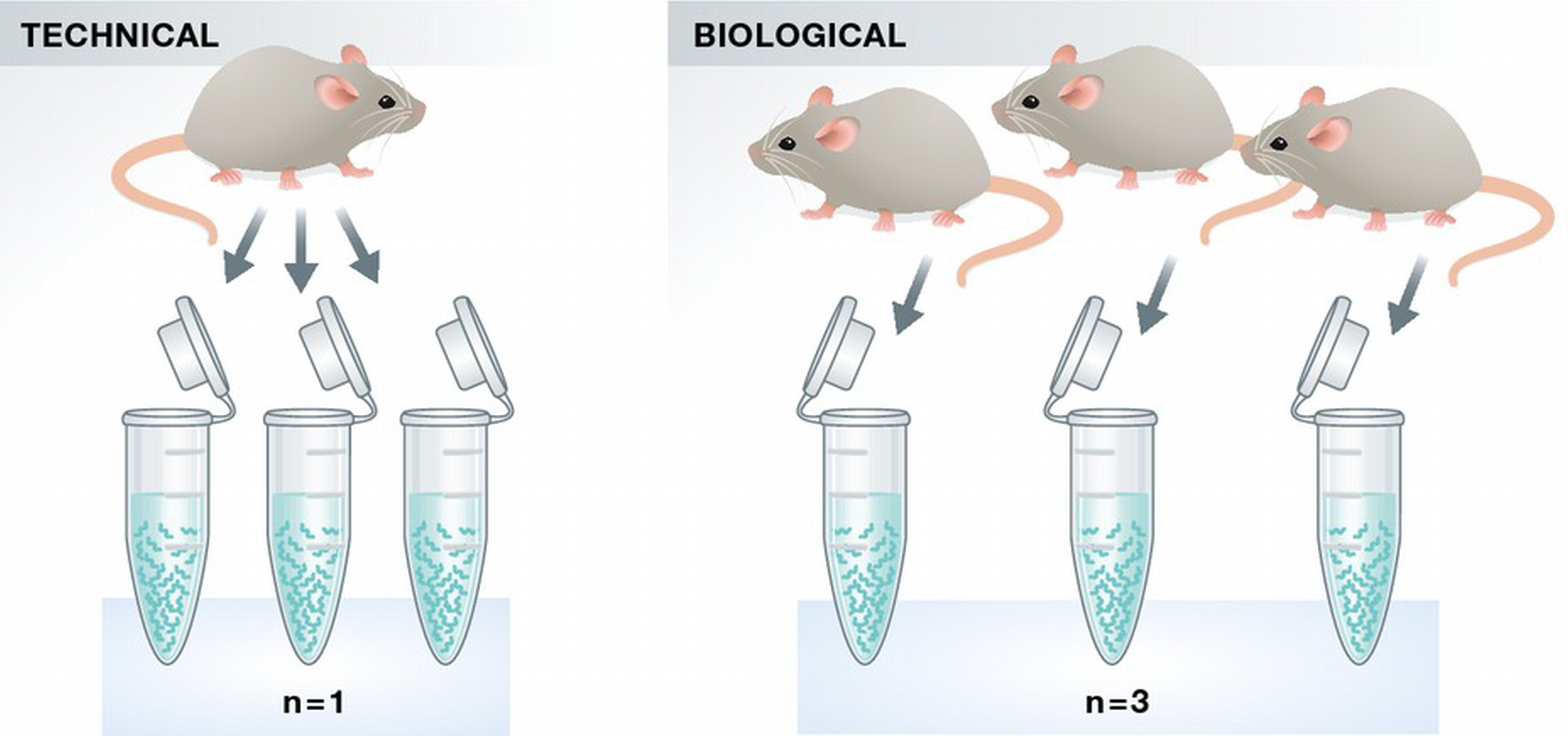
Biological vs technical replicates
Biological replicates are samples derived from independent biological sources.
They capture natural biological variability.
Examples:
different individuals
independent cell cultures
independent tissue samples
Technical replicates are repeated measurements of the same biological sample.
Examples:
different library preparations from the same RNA sample
sequencing the same library in multiple lanes
repeated sequencing runs of the same library
Simple rule:
3 different mice → biological replicates
3 libraries from the same RNA → technical replicates
|
adapted from Bernd Klaus, EMBO 2015 |
Side note: scRNA-seq
In single-cell RNA-seq experiments, the biological replicate is usually the sample or donor, not the individual cell. Thousands of cells from the same sample do not replace biological replication. Treating cells as replicates leads to pseudoreplication. In differential expression analysis, cells are typically aggregated per sample (“pseudobulk”) to restore the correct unit of replication.
Pseudoreplication
Treating non-independent samples as replicates leads to pseudoreplication.
Example:
one mouse → 3 libraries
treated as 3 samples → incorrect
Important
The number of libraries does not determine replication.
The number of independent experimental units does.
Questions: Are these samples technical replicates, biological replicates, or pseudoreplicates?
Three samples from the same patient at different time points (treated as independent samples)
1000 cells were isolated from a tumor sample. The cells were divided into three batches, and three RNA-seq libraries were prepared, sequenced, and analyzed independently.
RNA was extracted from a single mouse liver sample. Three independent RNA-seq libraries were prepared from this RNA extraction by 3 different people and sequenced separately.
Bone marrow pooled from 6 mice per group to form two samples.
Technical vs biological variability in RNA-seq
Modern RNA-seq protocols have low technical variability (SEQC Consortium 2014).
In contrast, biological variability is substantial and differs between samples,
and the statistical power of reliable differential expression analysis strongly depends on the number of biological
replicates (RNA 2016).
Important
Biological variability is typically much larger than technical variability.
→ Biological replication is more important than technical replicates.
Side note: scRNA-seq
In single-cell experiments, technical variability can be large due to capture efficiency, dropout events, and amplification bias. This is why scRNA-seq analysis typically includes additional steps such as cell filtering, normalization methods designed for sparse data, and sometimes pseudobulk aggregation.
Side note: total RNA-seq
Total RNA-seq often relies on rRNA depletion rather than poly(A) selection. The efficiency of rRNA removal can vary between samples and may influence the proportion of informative reads.
Replication and statistical power
Statistical power is the probability of detecting a true difference in gene expression between conditions.
Note
The desired power of the research experiment is usually above 80%.
In clinical studies, power might be required to be above 90%.
The statistical power of an RNA-seq experiment depends on:
number of biological replicates: 2 replicates → typically insufficient, 5-6 replicates → good power for many studies
effect size (magnitude of expression change): log2fc=3 easy to detect, log2fc=0.5 needs more power
biological variability within each condition: higher variability → lower power
sequencing depth: more reads → lower-expressed genes are detected
Important
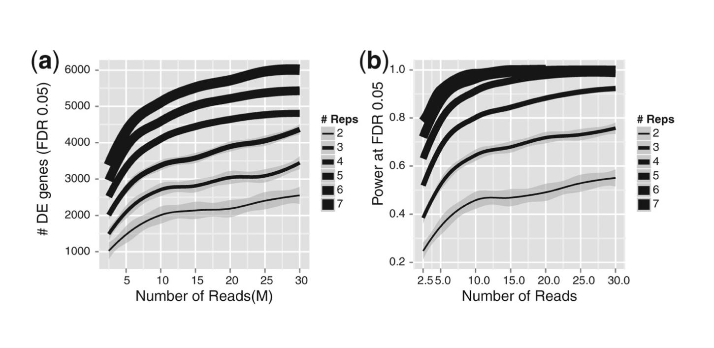
Increasing the number of biological replicates improves power more than increasing sequencing depth.
|
(a) Increase in biological replication significantly increases the number of DE genes identified. Numbers of sequencing reads have a diminishing return after 10 M reads. Line thickness indicates depth of replication, with 2 replicates the darkest and 7 replicates the lightest. The lines are smoothed averages for each replication level, with the shaded regions corresponding to the 95% confidence intervals. |
Overpowered vs underpowered experiment
If all other parameters remain the same,
a larger experiment will have more power than a smaller experiment.
However, if an experiment is too large and
a smaller experiment would have achieved the same
statistical result, the experiment is overpowered.
On the other hand, if an experiment is too small, it may be underpowered.
Warning
Both underpowered and overpowered experiments waste subjects, money, time and effort, and are potentially unethical.
Side note: scRNA-seq
Increasing the number of cells per sample improves cell-type resolution but does not increase statistical power for detecting differential expression between conditions. Power depends primarily on the number of biological samples (donors or experimental units).
Side note: ONT RNA-seq
For isoform-level analyses using long reads, statistical power depends strongly on read depth per transcript, because many isoforms are rare and require sufficient long-read coverage to be detected reliably.
Number of replicates in RNA-seq experiments
|
Statistical properties of edgeR (exact) as a function of log2FC threshold, T, and the number of replicates, nr. (A) The fraction of all (7126) genes called as SDE as a function of the number of replicates nr. (B) Mean true positive rate (TPR) as a function of nr for four thresholds (solid curves). (C) Mean TPR as a function of T for nr (solid curves). (D) The number of genes called as TP, FP, TN, and FN as a function of nr. |
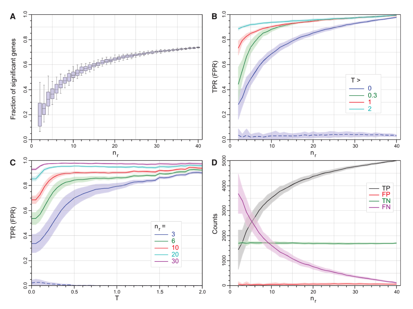
The study showed that:
With 3 replicates: many differentially expressed genes were missed (Fig A - <30% SDEs identified); especially many lower expressed genes were missed (Fig B - TPR = 0.8 for log2FC > 1).
With 6 replicates: most strong signals were detected (Fig B - TPR = 0.87 for log2FC > 1; TPR = 0.8 for log2FC > 0.5)
More than 10 replicates might be required to detect small expression changes (Fig. C - TPR = 0.9 for log2FC > 0.3, or FC = 1.24)
Side note: scRNA-seq
In many scRNA-seq studies, only a few donors are sequenced but thousands of cells are obtained per donor. While this enables detailed cell-type characterization, robust differential expression between biological conditions still requires multiple independent samples.
Side note: ONT RNA-seq
Long-read RNA sequencing experiments sometimes include fewer biological replicates due to cost and sequencing throughput. In such cases, results should often be interpreted as exploratory, especially for differential expression analyses.
When the number of replicates is limited
In practice, RNA-seq experiments often use a small number of biological replicates due to cost or sample availability.
A large-scale analysis (Degen & Medo, 2025) showed that small-cohort experiments frequently produce results that do not replicate well.
|
DEG performance metrics as a function of the cohort size. Each symbol summarizes the median of 100 cohorts. All panels show results using the DESeq2 Wald test with abs(log2FC) above 1. |
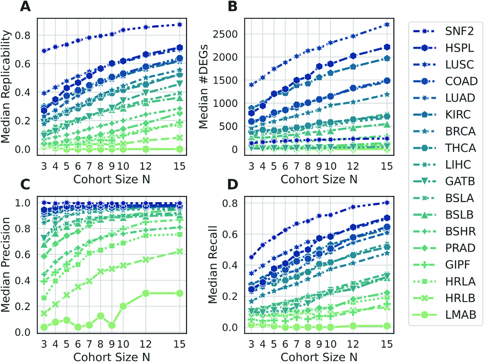
Key observations:
Small cohorts (N ≤ 3) show low replicability (Fig A, except SNF2 dataset)
Precision can be high even with a few samples (Fig C & D)
Recall is low, so many true differences are missed (for all data sets except SNF2, recall is below 0.5 for N<7)
→ Small experiments detect mainly strong effects
|
Heat maps and fold change estimates for SNF2 and LMAB data sets. |
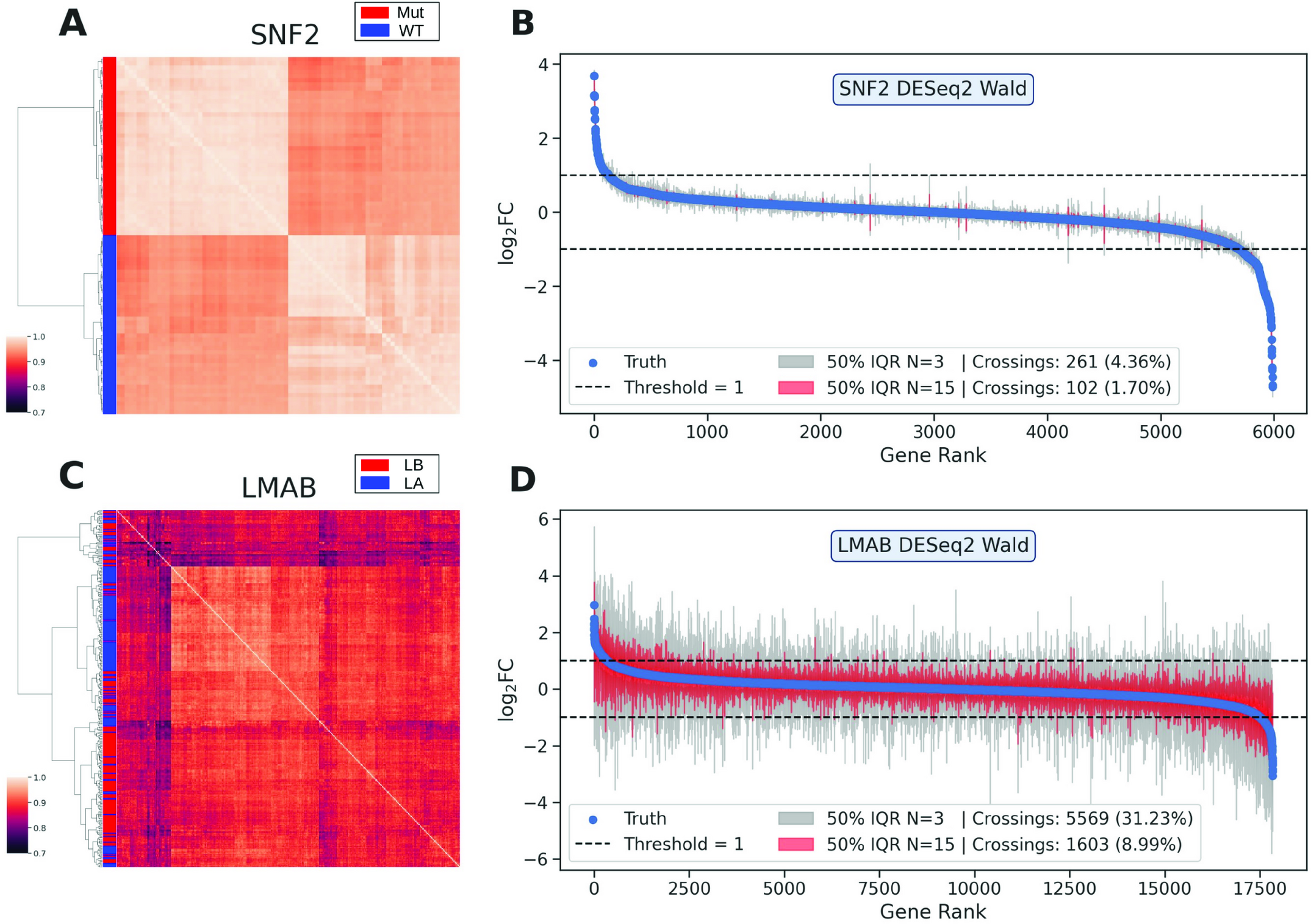
A second analysis shows that effect size estimates become unstable when replication is low.
Key observation:
In heterogeneous datasets, fold-change estimates vary widely (LMAB dataset: samples were derived from heterogeneous tumor tissues) → estimates can be inflated or underestimated
Homogeneous systems behave more consistently (SNF2 data set: cell colonies) → variability depends on the biological system
Practical implications
When replication is limited:
treat results as hypothesis-generating
interpret results cautiously (especially in heterogeneous samples)
focus on genes with larger effect sizes
validate key findings independently
What does it mean “focus on large effect size”?
That means that instead of testing the null hypothesis log2FC=0
test for abs(log2FC) > lfcThreshold (e.g., =1).
DESeq2 implementation:
results(dds, lfcThreshold = 1)
Thus, instead of asking
Is the gene differentially expressed?
you ask
Is the fold change larger than a biologically meaningful threshold?
Rule of thumb for RNA-seq experiments
2 replicates → insufficient
3 replicates → minimum
5–6 replicates → good / recommended
10+ replicates → robust
Small experiments detect only large expression changes;
subtle effects require more replication.
:::{admonition} Warning on replicate correlation :class: warning
High replicate concordance (e.g. high correlation) does not replace biological replication.
Similarity reflects consistency, but not the variability required for statistical inference.
Recommended number of sequencing reads
For bulk RNA-seq differential expression (human/mouse):
~30 million mapped reads per sample (ENCODE guideline)
→ typically ~35–40 million sequenced reads
Typical recommendations:
Application |
Reads per sample |
|---|---|
Gene-level differential expression |
35–40 million |
Isoform / splicing analysis |
50–100 million |
Low-abundance transcripts |
>100 million |
Sequencing depth affects:
detection of low-expressed genes
precision of expression estimates
isoform resolution
Important
Increasing sequencing depth improves sensitivity,
but does not replace biological replication.
More reads help detect genes; more samples help detect differences.
Side note: scRNA-seq
Sequencing depth is typically expressed per cell rather than per sample. Typical recommendations for droplet-based scRNA-seq range from 20,000 to 50,000 reads per cell for gene-level analysis, although deeper sequencing may be required for rare transcripts.
Randomization and batch effects
RNA-seq experiments include both:
biological factors (e.g. treatment, sex, genotype)
technical factors (e.g. batch, sample processing order, library prep, sequencing lane, flowcell)
If technical factors are aligned with biological conditions,
they become confounded, and biological effects cannot be separated from technical variation.
“Confounding” definition
Confounding (Adjective): Used to describe something that causes confusion or bewilderment (e.g., “the confounding details”) (Merriam-Webster dictionary).
In statistics, confounding means mixing two effects so they cannot be separated.
In RNA-seq: if a technical factor (e.g. batch) is aligned with the biological condition, you cannot tell which one caused the difference.
Example of confounding (bad design)
Lane |
Samples |
|---|---|
Lane 1 |
control, control, control |
Lane 2 |
treated, treated, treated |
→ lane effect = treatment effect
→ impossible to distinguish
Proper randomization (good design)
Lane |
Samples |
|---|---|
Lane 1 |
control, treated, control |
Lane 2 |
treated, control, treated |
→ technical variation is distributed across conditions
Important
Randomize samples across all experimental steps:
RNA extraction
library preparation
sequencing
Batch effects in RNA-seq
A batch is a group of samples processed together under the same technical conditions during an experimental step.
How to detect potential batches?
Ask whether technical conditions differed across samples:
Were all RNA isolations performed on the same day?
Were all library preparations performed on the same day?
Did the same person perform the RNA isolation/library preparation for all samples?
Did you use the same reagents for all samples?
Did you perform the RNA isolation/library preparation in the same location?
If any answer is “No”, then technical batches may exist.
Having batches does not automatically mean there is a batch effect problem.
Batches are common and often unavoidable in real experiments.
Batches exist but are randomized (good design)
Batch |
Samples |
|---|---|
Batch 1 |
control, treated |
Batch 2 |
control, treated |
Batch 3 |
control, treated |
Batch 4 |
control, treated |
Here, batch and condition are independent.
Batch effects may exist but can be separated from the biological effect.
Solution: batch can be ignored if its effect is small or modeled (in DESeq, design = ~ batch + condition)
Batch is fully confounded with condition (fatal design error):
Batch |
Samples |
|---|---|
Batch 1 |
treated, treated |
Batch 2 |
control, control |
Batch 3 |
treated, treated |
Batch 4 |
control, control |
treatment effect = batch effect
The biological condition is perfectly confounded with the batch variable.
No statistical method can separate these effects.
Batch effect rule
Batch effects are problematic only when they are correlated with the biological condition.
Blocking or How to control known variation
While randomization protects against factors that are not modeled or cannot be modeled,
blocking is used when a known source of variation exists
(for example, library preparation batches or patients).
Blocking explicitly models batch as a variable.
Even if batches contain the same number of samples per condition, processing order can introduce bias (e.g., reagent degradation, operator fatigue - technical factors that cannot be modeled).
Example: systematic bias caused by processing order
Batch 1
Sample |
treated |
treated |
treated |
control |
control |
control |
|---|---|---|---|---|---|---|
Processing order |
1 |
2 |
3 |
4 |
5 |
6 |
Batch 2
Sample |
control |
control |
control |
treated |
treated |
treated |
|---|---|---|---|---|---|---|
Processing order |
1 |
2 |
3 |
4 |
5 |
6 |
Since the processing order can introduce unknown bias that cannot be modeled, randomization has to be applied.
Randomized processing order
Batch 1
Sample |
control |
treated |
control |
treated |
treated |
control |
|---|---|---|---|---|---|---|
Processing order |
1 |
2 |
3 |
4 |
5 |
6 |
Batch 2
Sample |
treated |
control |
treated |
control |
control |
treated |
|---|---|---|---|---|---|---|
Processing order |
1 |
2 |
3 |
4 |
5 |
6 |
Randomizing the processing order distributes potential technical variation (e.g. reagent degradation or operator effects) across biological conditions.
Key message
Randomize what you cannot control,
block what you can control (using batch in statistical model: design = ~ batch + condition).
Factorial designs and interactions
Many RNA-seq experiments involve more than one biological factor.
Example:
Treatment |
Sex |
|---|---|
control |
male |
control |
female |
drug |
male |
drug |
female |
Each factor has two levels, producing four experimental groups.
This is a 2 × 2 factorial design.
Such a design allows testing:
Main effect of treatment - Does the treatment change gene expression?
Main effect of sex - Do males and females differ in gene expression?
Interaction between treatment and sex - Does the treatment affect males and females differently?
An interaction occurs when the effect of one factor depends on the level of another factor.
Interaction = difference of differences:
(treated_males − control_males) − (treated_females − control_females)
Example for a specific gene in an RNA-seq experiment:
Sex |
Control |
Drug |
|---|---|---|
Male |
low expression |
high expression |
Female |
low expression |
unchanged |
→ treatment effect exists only in males
→ suggests treatment × sex interaction
That is,
(treated_male − control_male) ≠ (treated_female − control_female)
In RNA-seq analysis, for each gene, a model such as
design = ~ sex + treatment + sex:treatment
tests three things:
term |
interpretation |
|---|---|
sex |
baseline difference between males and females |
treatment |
treatment effect averaged across sexes |
sex:treatment |
whether treatment effect differs between sexes |
The pattern suggests a potential treatment × sex interaction, because the treatment increases expression in males but not in females. However, whether this interaction is statistically significant depends on the variability between replicates and the number of samples.
Practical implications
Factorial designs allow researchers to:
test multiple biological hypotheses in a single experiment
increase experimental efficiency
avoid performing multiple separate experiments
However, factorial designs require sufficient replication in each experimental group to reliably estimate effects and interactions.
When multiple factors are studied, the number of experimental groups increases because each combination of factor levels must be measured.
If each group contains N biological replicates, the total number of samples becomes:
total samples = number of groups × N
For example, for a 2 × 2 factorial design (4 experimental groups):
Replicates per group |
Total samples |
|---|---|
3 |
12 |
5 |
20 |
8 |
32 |
In RNA-seq experiments, factorial designs are common when studying treatment effects across sex, genotype, time points, or environmental conditions.
Practical rule of thumb for factorial design
3 biological replicates per group → minimum (exploratory; sufficient mainly for homogeneous systems)
5–6 per group → reasonable for main effects and strong interactions
8+ per group → more reliable detection of moderate to small interactions
Key design rules for RNA-seq experiments
Define the experimental unit correctly
Use sufficient biological replication (3 minimum, preferably 5–6)
Randomize samples across all experimental steps
Record and model batch effects when present
Ensure adequate sequencing depth (~30M mapped reads)
Use factorial designs when studying multiple factors
Important
Replication determines power.
Design determines whether results are interpretable.
References
RNA-seq experimental design and replication
Schurch NJ. RNA. 2016.
How many biological replicates are needed in an RNA-seq experiment and which differential expression tool should you use?
https://www.ncbi.nlm.nih.gov/pmc/articles/PMC4878611/Liu Y. Bioinformatics. 2014.
RNA-seq differential expression studies: more sequence or more replication?
https://www.ncbi.nlm.nih.gov/pmc/articles/PMC3904521/Tarazona S. Genome Research. 2011.
Differential expression in RNA-seq: a matter of depth or replication?
https://genome.cshlp.org/content/21/12/2213SEQC Consortium. Nature Biotechnology. 2014.
A comprehensive assessment of RNA-seq accuracy, reproducibility and information content by the Sequencing Quality Control Consortium.
https://pmc.ncbi.nlm.nih.gov/articles/PMC4321899Degen R. PLOS Computational Biology. 2025.
Replicability of RNA-seq differential expression results with small sample sizes.
https://journals.plos.org/ploscompbiol/article?id=10.1371/journal.pcbi.1011630Antoszewski M. Methods. 2025.
A practical guide to designing RNA-seq experiments.
https://www.sciencedirect.com/science/article/pii/S2001037025005525
Statistical power and experimental design
Lieber RL. Journal of Orthopaedic Research. 1990.
Statistical significance and statistical power in hypothesis testing.
http://muscle.ucsd.edu/More_HTML/papers/pdf/Lieber_JOR_1990.pdfBiau DJ. Emergency Medicine Journal. 2003.
An introduction to power and sample size estimation.
https://emj.bmj.com/content/20/5/453Button KS. Nature Reviews Neuroscience. 2013.
Power failure: why small sample size undermines the reliability of neuroscience.
https://www.ncbi.nlm.nih.gov/pmc/articles/PMC5367316/Gigerenzer G. Psychological Science. 2004.
Mindless statistics.
http://library.mpib-berlin.mpg.de/ft/gg/GG_Mindless_2004.pdf
Guidelines and educational resources
ENCODE Consortium.
Guidelines and Best Practices for RNA-seq.
https://www.encodeproject.org/documents/cede0cbe-d324-4ce7-ace4-f0c3eddf5972/@@download/attachment/ENCODE%20Best%20Practices%20for%20RNA_v2.pdfStatistics Knowledge Portal – Design of Experiments.
https://www.jmp.com/en/statistics-knowledge-portal/design-of-experiments/key-design-of-experiments-concepts/key-principles-of-experimental-designExperimental Design Assistant (NC3RS).
https://eda.nc3rs.org.uk/experimental-designStatistics Done Wrong – Underpowered statistics.
https://www.statisticsdonewrong.com/power.html