Hands-on: Reviewing some R basics
In this section, we will review:
RStudio/POSIT software usage
R basics.
RStudio
What is RStudio?
Free and open source IDE (Integrated Development Environment) for R, Python
Available for Windows, Mac OS and LINUX
We will use a local RStudio server running a singularity container. It uses Tidyverse Rocker image.
# Download the bash script that installs the singularity container and run it in the localserver
wget https://raw.githubusercontent.com/biocorecrg/RNAseq_coursesCRG_2026/refs/heads/master/run_rstudio.sh
bash run_rstudio.sh
In your browser, type the following url: http://localhost:8787/
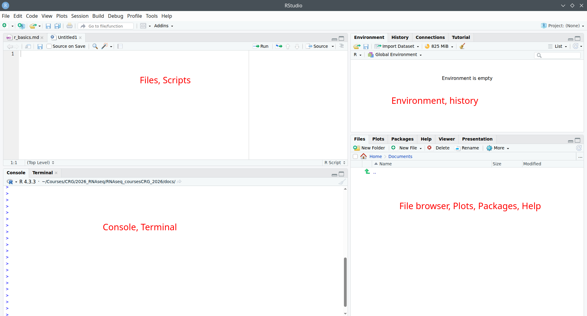
Panels
When you open RStudio, you will see 3-4 panels:
top-left: scripts and files
bottom-left: R console Linux-line terminal / command-line
top-right: environment, history, connections, tutorial
bottom-right: tree of folders and files, plots/graphs window, packages, help window, viewer, presentation
Shortcuts
RStudio provides a variety of shortcuts to make user interaction smoother.
Click Alt + Shift + K to display all available shortcuts.
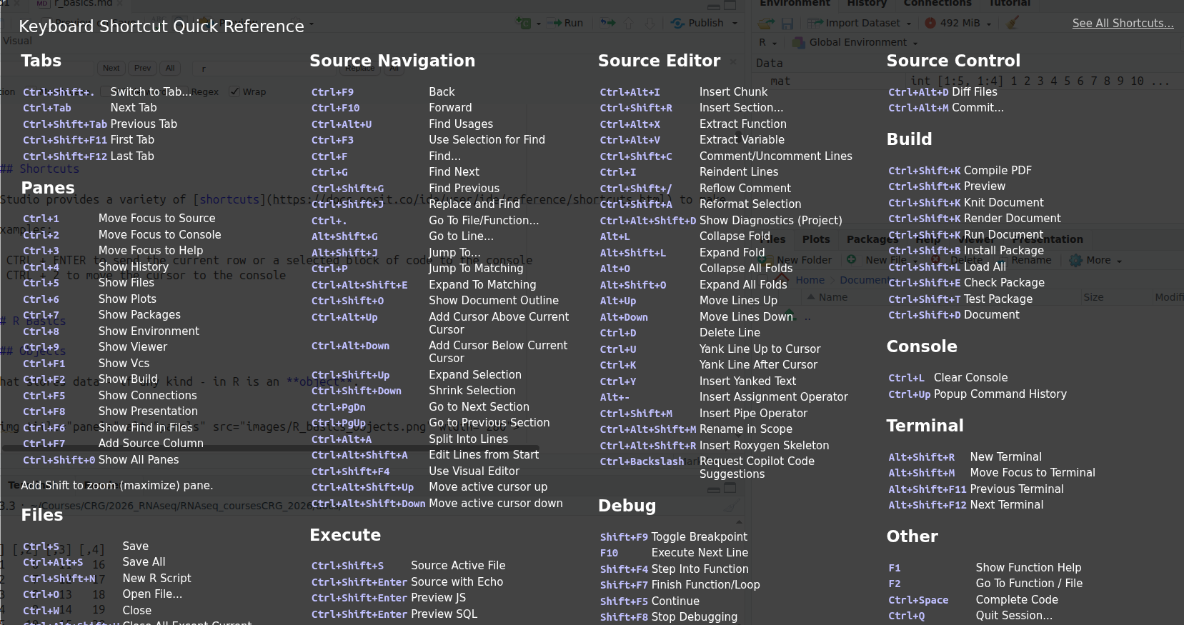
Examples:
CTRL + ENTER to send the current row or a selected block of code to the console
CTRL + 2 to move the cursor to the console
https://docs.posit.co/ide/user/ide/guide/code/projects.html
Tip
If you start using RStudio IDE for your work, please refer to the (great) official documentation, for example:
R Basics
Objects
What stores data - of any kind - in R is an object.
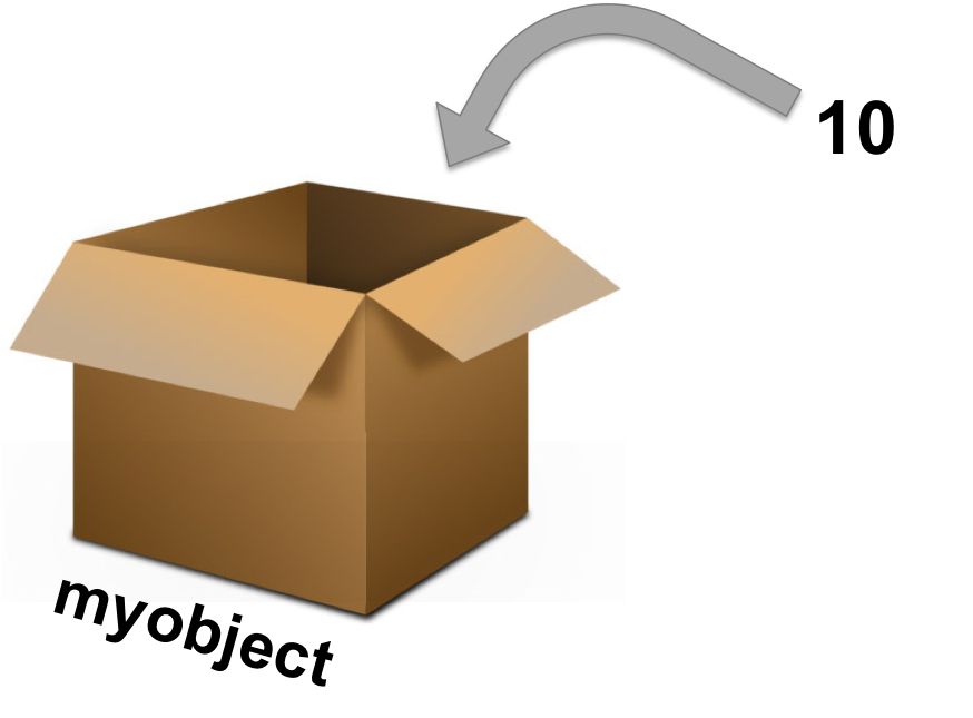
Assignment operators (how to assign data to the object):
<- or =
Mostly the same but, to avoid confusions:
Use <- for assignments
Keep = for functions arguments
Assigning a value to the object B:
B <- 10
B + 10
B unchanged !!
Reassigning: modifying the content of an object:
B <- B + 10
B changed !!
You can see the objects you created in the environment panel (upper right).
Note
Naming an object in R is flexible. You should nevertheless follow a few base rules:
You can use:
Letters (note that object names case sensitive: A and a are NOT the same)
Numbers (exception: the object name cannot start with a number)
Underscores _
You cannot use:
Spaces
Most special characters
Data types and data structures
Data types
Each object has a data type:
Numeric (number - integer or double)
Character (text)
Logical (TRUE / FALSE)
Factors (categorical variables)
Numeric: numbers, floats
number_object <- 10
mode(number_object)
typeof(number_object)
str(number_object)
Character: text, strings of characters
text_object <- "word"
mode(text_object)
typeof(text_object)
str(text_object)
Logical: boolean values (TRUE or FALSE)
logical_object <- TRUE
mode(logical_object)
typeof(logical_object)
str(logical_object)
Factor: used to work with categorical variables. For example, in statistical modeling or graphing.
Creating a factor starts by creating an object, that is then converted to a factor.
factor_object <- factor(text_object)
mode(factor_object)
typeof(factor_object)
str(factor_object)
Data structures
The main data structures in R are:
Vector
Matrix
Data frame
List
Vectors
Vectors are one-dimensional and contain a single data type.
Create a numeric vector:
a <- c(1, 2, 3, 4, 5, 6)

# same as:
a <- 1:6
Note
shorta <- 1
same as:
shorta <- c(1)
shorta is a vector of 1-element.
Check the length of (i.e. number of elements) a vector:
length(a)
You can extract elements of a vector using the slicing operator (the square bracket) [ ]:
Extract 1st and 3rd elements of a:
a[c(1,3)]
Extract all but the first element:
a[-1]
Create a second numeric vector, and check which elements of that second vector are also present in a using operator %in%:
b <- 3:8

b[b %in% a]
Tip
Table of comparison and logical operators that can be used for data selection and filtering:
Operator |
Description |
|---|---|
< |
less than |
<= |
less than or equal to |
> |
greater than |
>= |
greater than or equal to |
== |
exactly equal to |
!= |
not equal to |
!x |
not x |
x|y |
x OR y |
x&y |
x AND y |
%in% |
checks if an element belongs to a vector |
You can replace one element of a vector by pointing to its position, e.g.:
b[2] <- 10
Matrices
Matrices are two-dimensional and can only contain one data type.
Create a numeric matrix:
# define number of rows
mat <- matrix(1:100, nrow=4)

# define number of columns
mat <- matrix(1:100, ncol=4)
Check dimensions (i.e. number of rows and number of columns) of a matrix:
# Number of rows
nrow(mat)

# Number of columns
ncol(mat)

# Dimensions (first element is the number of rows, second element is the number of columns)
dim(mat)
Display the first or last rows with head or tail:
# first 6 rows (default)
head(mat)

# first 10 rows
head(mat, n=10)

# last 6 rows
tail(mat)
You can extract rows and columns of a matrix using the slicing operator (square bracket [ ] and their position/index:
# first row
mat[1,]

# row 1 and 3
mat[c(1,3),]

# first column
mat[,1]

# column 2 and 3
mat[,c(2, 3)]

# or mat[,2:3]
Note
The left item of the square bracket always corresponds to the row, while the right item always corresponds to the column:
mat[row_index, colum_index]
Data frames
Data frames are two-dimensional and can contain several data types (column-wise: one column will have a single data type).
Create a three-column data frame :
Name: character columnAge: numeric columnVegetarian: logical column
# create data frame
df <- data.frame(c("Maria", "Juan", "Alba", "Xavier", "Lara", "Max"),
        c(23, 25, 31, 28, 36, 34),
        c(TRUE, TRUE, FALSE, FALSE, TRUE, FALSE))

# add column names
colnames(df) <- c("Name", "Age", "Vegetarian")

# do both steps at once
df <- data.frame(Name=c("Maria", "Juan", "Alba", "Xavier", "Lara", "Max"),
        Age=c(23, 25, 31, 28, 36, 34),
        Vegetarian=c(TRUE, TRUE, FALSE, FALSE, TRUE, FALSE))
Check dimensions (i.e. number of rows and number of columns) of a dataframe:
# Number of rows
nrow(df)

# Number of columns
ncol(df)

# Dimensions (first element is the number of rows, second element is the number of columns)
dim(df)
Check column names or row names:
colnames(df)

rownames(df)
You can extract rows - as with matrices - using the slicing operator: the square bracket [ ] df[1,]
You can extract columns of a data frame with:
Slicing operator []
Access using the column name:
df[,"Age"]Access using the column index (i.e. position):
df[,2]
Dollar sign $:
df$Age
Select rows of the data frame if the Age column is greater than 24:
df[df$Age > 24,]
Select rows of the data frame based on multiple conditions, for example, if the Age column is greater than 24 AND if Vegetarian is TRUE :
df[df$Age > 24 & df$Vegetarian == TRUE,]
Finally, select only columns of interest for your selection: in the following example, we extract the name of vegetarian people older than 24:
df[df$Age > 24 & df$Vegetarian == TRUE, "Name"]
Lists
Lists are one-dimensional: each element of a list can contain a different data structure!
mylist <- list(my_df=df,
              my_vector=b,
              my_matrix=mat)
The length of a list gives you the number of elements.
length(mylist)
You can extract elements of a list (and apply functions on them) using the double square brackets [[ ]].
# extract third element of the list with the index...
mylist[[3]]
# or the name
mylist[["my_matrix"]]
mylist$my_matrix

# check dimensions of the third element
dim(mylist[[3]])
Paths and directories
Get/show the path of the current directory (i.e. working directory) with getwd (get working directory):
getwd()
Change working directory with setwd (set working directory).
Go to a directory giving the absolute path:
setwd("~")
# the home directory is likely different for each of you, but it could be like /users/username
Note
~ is a shortcut to your home directory
Now that you are in your home directory, you can create an rnaseq_course directory (if you have not created a folder for the course yet) and an r_basics directory:
dir.create("rnaseq_course/r_basics", recursive=TRUE)
Go to the newly created directory using the relative path:
setwd("./rnaseq_course/r_basics")

# which is equivalent to
setwd("~/rnaseq_course/r_basics")
You are now in: “~/rnaseq_course/r_basics”
Move one directory “up” the tree:
setwd("..")

# and move back to r_basics
setwd("r_basics")
You are now back to: “~/rnaseq_course/r_basics”
Missing values
NA (Not Available) is a recognized element in R.
Finding missing values in a vector:
# Create vector with a missing value
x <- c(4, 2, 7, NA)

# Find missing values in vector:
is.na(x)

# Remove missing values
na.omit(x)
x[ !is.na(x) ]
Some functions can deal with NAs, either by default, or with specific parameters:
x <- c(4, 2, 7, NA)

# default arguments: what happens?
mean(x)

# set na.rm=TRUE for the mean function to handle (in this case, ignore) missing values
mean(x, na.rm=TRUE)
In a matrix or a data frame, you can keep only rows where there are no NA values with:
# Create matrix with some NA values
mydata <- matrix(c(1:10, NA, 12:2, NA, 15:20, NA), ncol=3)

# Keep only rows without NAs
mydata[complete.cases(mydata), ]
# or
na.omit(mydata)
For additional information, you can check this R blogger post on missing/null values
Read in, write out
On vectors
Write the content of a vector in a file with write:
# create a vector
mygenes <- c("SMAD4", "DKK1", "ASXL3", "ERG", "CKLF", "TIAM1", "VHL", "BTD", "EMP1", "MALL", "PAX3")

# write to a file
write(x=mygenes,
        file="gene_list.txt")
You can specify a full or relative path where to write down a file:
# Write to home directory
write(x=mygenes,
        file="~/rnaseq_course/r_basics/gene_list.txt")

# Write to one directory up
write(x=mygenes,
        file="../gene_list.txt")
Read in a file into a vector object using scan:
# Read in file
scan(file="gene_list.txt")

# Save scanned data into an object k
k <- scan(file="gene_list.txt")
By default, the function scans for “double” (numeric) elements: it fails if the input contains characters.
If reading non-numeric data, you need to specify the type of data contained in the file:
# specify the type of data to scan
scan(file="gene_list.txt",
        what="character")
If the file is not in the current directory, you can provide a full or relative path.
For example, if the file is located in the home directory, read it as:
scan(file="~/gene_list.txt",
        what="character")

# here, we can read it as:

scan(file="~/rnaseq_course/r_basics/gene_list.txt", what="character")
Data frames or matrices
Read in a file as a data frame with read.table:
a <- read.table(file="file.txt")
You can convert it as a matrix, if needed, with:
a <- as.matrix(read.table(file="file.txt"))
Write a data frame or matrix to a file with write.table:
write.table(x=a,
        file="file.txt")
Useful arguments:
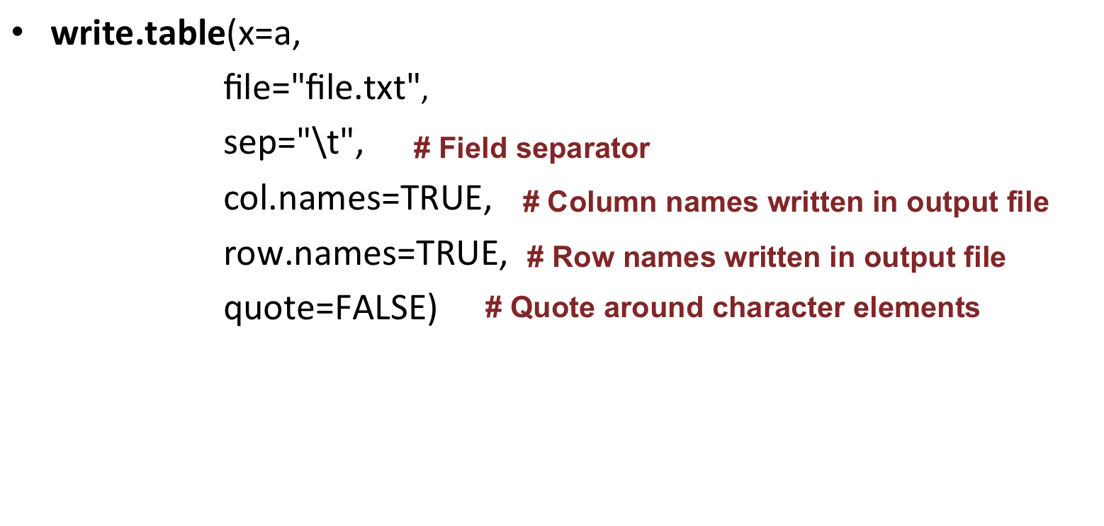
Note that sep=”\t” stands for tab-delimitation; if reading a .csv file, you can change to sep=”,” (or use the dedicated write.scv function!).
Install packages
R base
A set a standard packages which are supplied with R by default.
Example: package base (write, table, rownames functions), package utils (read.table, str functions), package stats (var, na.omit, median functions).
R contrib
All other packages:
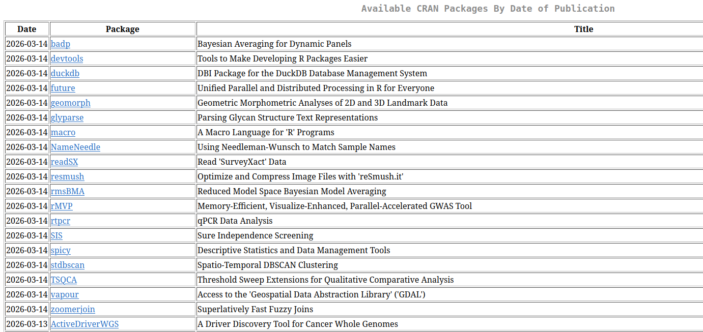
CRAN: Comprehensive R Archive Network
23422* packages available
find packages in https://cran.r-project.org/web/packages/
-
2361* packages available
find packages in https://bioconductor.org/packages
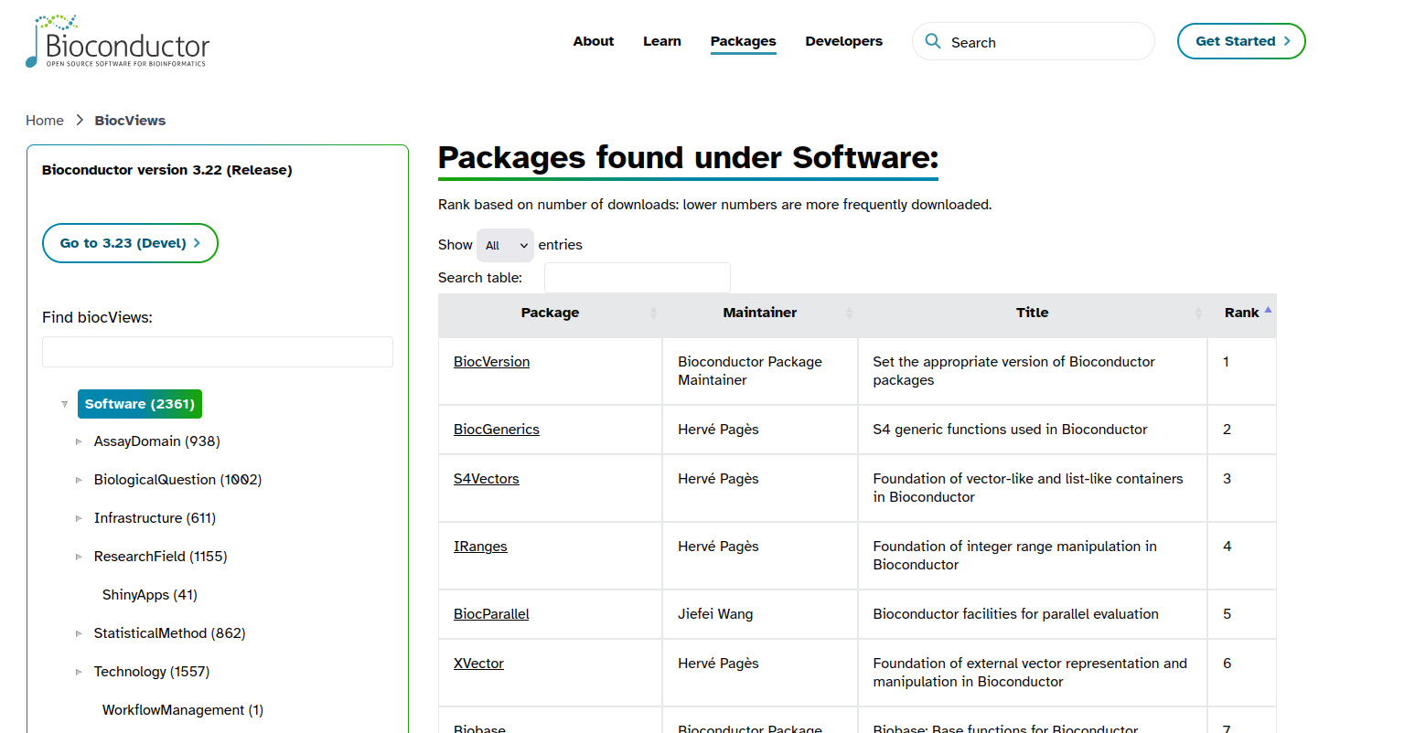
* As of March 2026
Install a CRAN package using install.packages:
install.packages('BiocManager', repos = 'http://cran.us.r-project.org', dependencies = TRUE)
Install a Bioconductor package using BiocManager::install:
library('BiocManager')
BiocManager::install('GOstats')
Exercises
Exercise 1
Create a numeric vector y containing numbers from 2 to 11 (both included).
How many elements are in y?
Show the 3rd and the 6th elements of y.
Show all elements of y that have a value inferior to 7.
Click to show correction
Create a numeric vector y containing numbers from 2 to 11 (both included).
y <- 2:11
or
y <- c(2, 3, 4, 5, 6, 7, 8, 9, 10, 11)
How many elements are in y?
length(y)
Show the 3rd and the 6th elements of y.
y[c(3,6)]
Show all elements of y that have a value inferior to 7.
y[y < 7]
Exercise 2
Create the vector x of 1000 random numbers from the normal distribution (see rnorm function).
What are the mean, median, minimum and maximum values of x?
Click to show correction
Create the vector x of 1000 random numbers from the normal distribution (see rnorm function).
x <- rnorm(1000)
What are the mean, median, minimum and maximum values of x?
mean(x); median(x); min(x); max(x)
or the more straightforward:
summary(x)
Exercise 3
Create vector y2 as: y2 <- c(1, 11, 5, 62, NA, 18, 2, 8, NA)
What is the sum of all elements in y2 ?
Which elements of y2 are also present in y?
Remove NA values from y2.
Click to show correction
Create vector y2 as:
y2 <- c(1, 11, 5, 62, NA, 18, 2, 8, NA)
What is the sum of all elements in y2 ?
sum(y2, na.rm = TRUE)
Which elements of y2 are also present in y?
y2[y2 %in% y]
Remove NA values from y2.
y2 <- na.omit(y2)
Exercise 4
Create the following data frame:
43 |
181 |
M |
34 |
172 |
F |
22 |
189 |
M |
27 |
167 |
F |
with :
row names: John, Jessica, Steve, Rachel
column names: Age, Height, Sex.
Then:
Check the structure of df with str().
Calculate the average age and height in df.
Change the row names of df so the data becomes anonymous
Use for example Patient1, Patient2, etc.
Write df to the file mydf.txt with write.table().
Explore parameters sep, row.names, col.names, quote.
Click to show correction
Create the following data frame wih
row names: John, Jessica, Steve, Rachel
column names: Age, Height, Sex.
df <- data.frame(Age=c(43, 34, 22, 27), Height=c(181, 172, 189, 167), Sex=c(“M”, “F”, “M”, “F”), row.names = c(“John”, “Jessica”, “Steve”, “Rachel”))
Check the structure of df with str().
str(df)
Calculate the average age and height in df.
mean(df$Age)
same as mean(df[,"Age"])
mean(df$Height)
same as mean(df[,"Height"])
Change the row names of df so the data becomes anonymous
Use for example Patient1, Patient2, etc.
rownames(df) <- c("Patient1", "Patient2", "Patient3", "Patient4")
Write df to the file mydf.txt with write.table().
Explore parameters sep, row.names, col.names, quote.
write.table(df, “mydf.txt”, sep=”\t”, row.names = TRUE, col.names = NA, quote = FALSE)
Exercise 5
Create a matrix called
gradesrepresenting 4 students (rows) and 3 subjects (columns: Math, Science, English) with the following values:Student 1: 85, 92, 78
Student 2: 70, 88, 95
Student 3: 99, 91, 89
Student 4: 60, 72, 68
Extract the Science grade for Student 3
Calculate the average score for Math across all 4 students
Click to show correction
Create a matrix called
gradesrepresenting 4 students (rows) and 3 subjects (columns: Math, Science, English) with the following values:Student1: 85, 92, 78
Student2: 70, 88, 95
Student3: 99, 91, 89
Student4: 60, 72, 68
grades <- matrix(c(85, 92, 78, 79, 88, 95, 99, 91, 89, 60, 72, 68),
                nrow=4,
                byrow=TRUE,
                dimnames=list(c("Student1", "Student2", "Student3", "Student4"), c("Math", "Science", "English"))
                )
Extract the Science grade for Student 3
grades["Student3", "Science"]
Calculate the average score for Math across all 4 students
mean(grades[,"Math"])