Hands-on: Pre-processing and Quality Control of Raw Sequencing Data
Data for this course and SRA download
The Sequence Read Archive (SRA) at NCBI is a public repository of raw sequencing data. It is the primary source for publicly available datasets to use for practice, benchmarking, or reproduction of published results.
SRA Accession Types:
Prefix |
Level |
Example |
|---|---|---|
|
BioProject — the overall study |
PRJNA257197 |
|
BioSample — a biological specimen |
SAMN03254300 |
|
Experiment — library preparation metadata |
SRX123456 |
|
Run — the actual sequencing reads |
SRR1553607 |
The SRR Run accession is what you need to download reads. A single experiment (SRX) may have multiple runs (SRR). The data that will be using for the hands-on exercises is from GEO data set GSE76647. Specifically, it contains Homo sapiens samples from differentiated (5-day differentiation) and undifferentiated primary keratinocytes. Additionally, some samples underwent a knock-down of the FOXC1 gene.
We could try to download these datasets from SRA directly but due to time constrains, we have already prepared fastq files that correspond to chromosome 6 only. You will find them in the data directory (* ~/RNAseq_coursesCRG_2026/docs/data/reads/*) within the repository of the course.
Raw Data QC
Before any downstream analysis (alignment, read count, differential expression, functional enrichment), it is critical to assess the quality of raw sequencing reads and pre-process them accordingly. Poor-quality data can introduce errors that propagate through the entire pipeline.
Pre-processing includes:
Raw data QC:
Quality control of initial reads
Contamination checks
Read pre-processing:
Adapter trimming
Filtering out low-quality reads/base positions
rRNA removal (where applicable)
Tools Overview
Tool |
Purpose |
|---|---|
FastQC |
Per-read quality metrics |
FastQ Screen |
Contamination screening against reference genomes |
Kraken2 |
Taxonomic classification to detect biological contamination |
MultiQC |
Aggregates reports from all tools into one summary |
FastQC
FastQC is the standard first-pass QC tool for sequencing reads. It reads FASTQ files (also in gzipped format) and produces an HTML report with multiple modules, each assessing a different aspect of read quality.
Key metrics assessed:
Per-base sequence quality (Phred scores)
Per-sequence quality scores
Per-base sequence content (A/T/G/C composition)
Per-sequence GC content
Per-base N content
Sequence length distribution
Sequence duplication levels
Overrepresented sequences
Adapter content
Reminder — Phred quality scores
Phred scores (Q scores) encode the probability of a base-calling error:
Phred Score |
Error Probability |
Accuracy |
|---|---|---|
Q10 |
1 in 10 |
90% |
Q20 |
1 in 100 |
99% |
Q30 |
1 in 1,000 |
99.9% |
Q40 |
1 in 10,000 |
99.99% |
Reads are generally considered good quality if the median Phred score is ≥ Q30 across most bases.
Running FastQC
# Run FastQC on a single file
fastqc sample.fastq.gz

# Run on multiple files
fastqc sample1.fastq.gz sample2.fastq.gz

# Specify output directory
fastqc -o ./fastqc_results/ sample.fastq.gz

# Use multiple threads (faster for large files)
fastqc -t 4 -o ./fastqc_results/ *.fastq.gz
Output files
For each sample, two files are excepted:
sample_fastqc.html     # Visual HTML report with bar charts
sample_fastqc.zip      # Zip file with graphs and results in txt
Hands-on: FastQC
# Go to the "quality_control" folder
mkdir ~/RNAseq_coursesCRG_2026/raw_qc
cd ~/RNAseq_coursesCRG_2026/raw_qc

# Run FastQC for one sample
$RUN fastqc ~/RNAseq_coursesCRG_2026/docs/data/reads/SRR3091420_1_chr6.fastq.gz -o .

# Run for all samples
$RUN fastqc ~/RNAseq_coursesCRG_2026/docs/data/reads/*.fastq.gz -o .

# Check output
ls .
Display the results in a browser:
firefox SRR3091420_1_chr6_fastqc.html &
You can also extract the zip archive to access results in text format:
# Extract
unzip SRR3091420_1_chr6_fastqc.zip

# Remove remaining .zip file
rm SRR3091420_1_chr6_fastqc.zip

# Display content of directory
ls SRR3091420_1_chr6_fastqc

# File fastqc_data.txt contains the results in text format
less SRR3091420_1_chr6_fastqc/fastqc_data.txt
Interpreting Key Plots
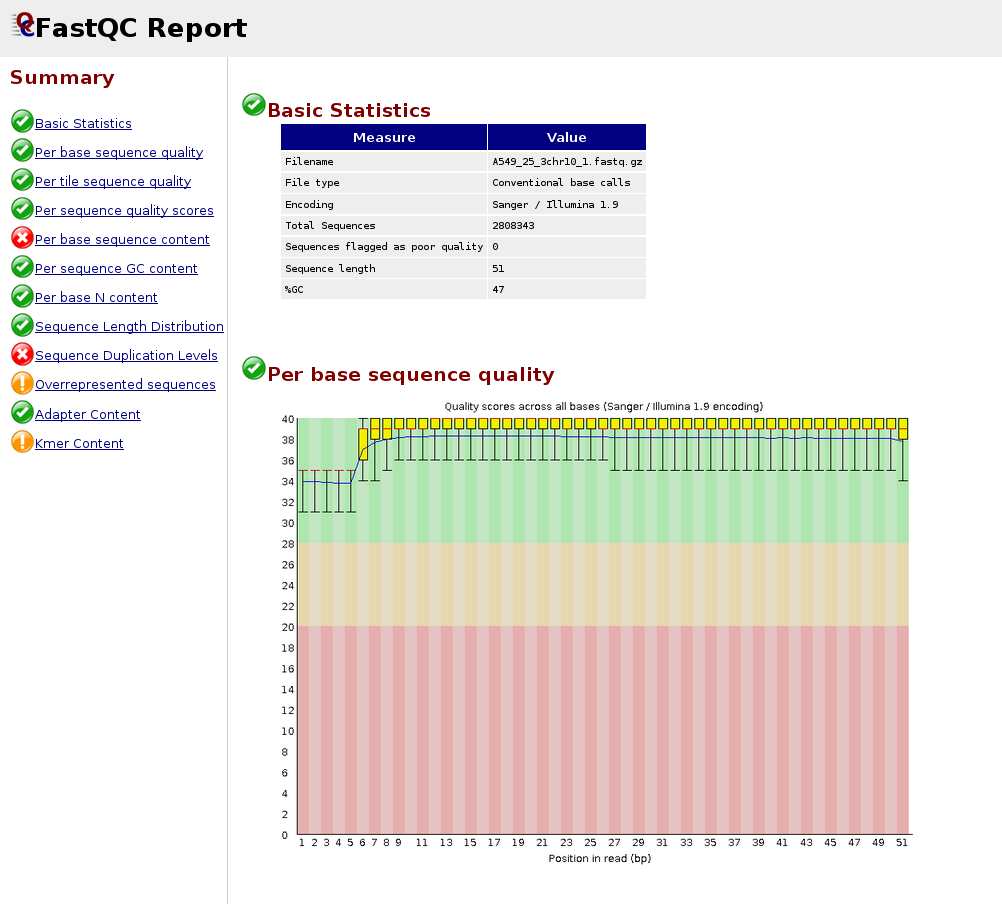
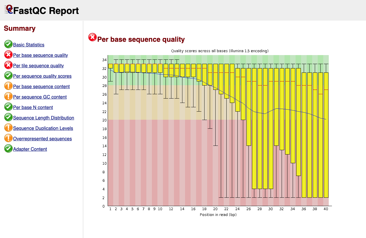
1. Per Base Sequence Quality
Good: Box plots remain in the green zone (Q > 28)
Warning: Boxes drop into yellow (Q 20–28)
Fail: Boxes drop into red (Q < 20)
Common pattern: quality drops at the 3’ end — this is normal for Illumina data
Below is an example of a good quality dataset (top) and a poor quality dataset (bottom). In the latter, the average quality drops dramatically towards the 3’-end.
|
Figure 1: Good quality per base sequence |
|
Figure 2: Bad quality per base sequence |
2. Per Sequence GC Content
Should follow a normal bell-shaped curve
A shifted peak may indicate contamination or adapter dimers
Bimodal distribution = likely contamination from another organism
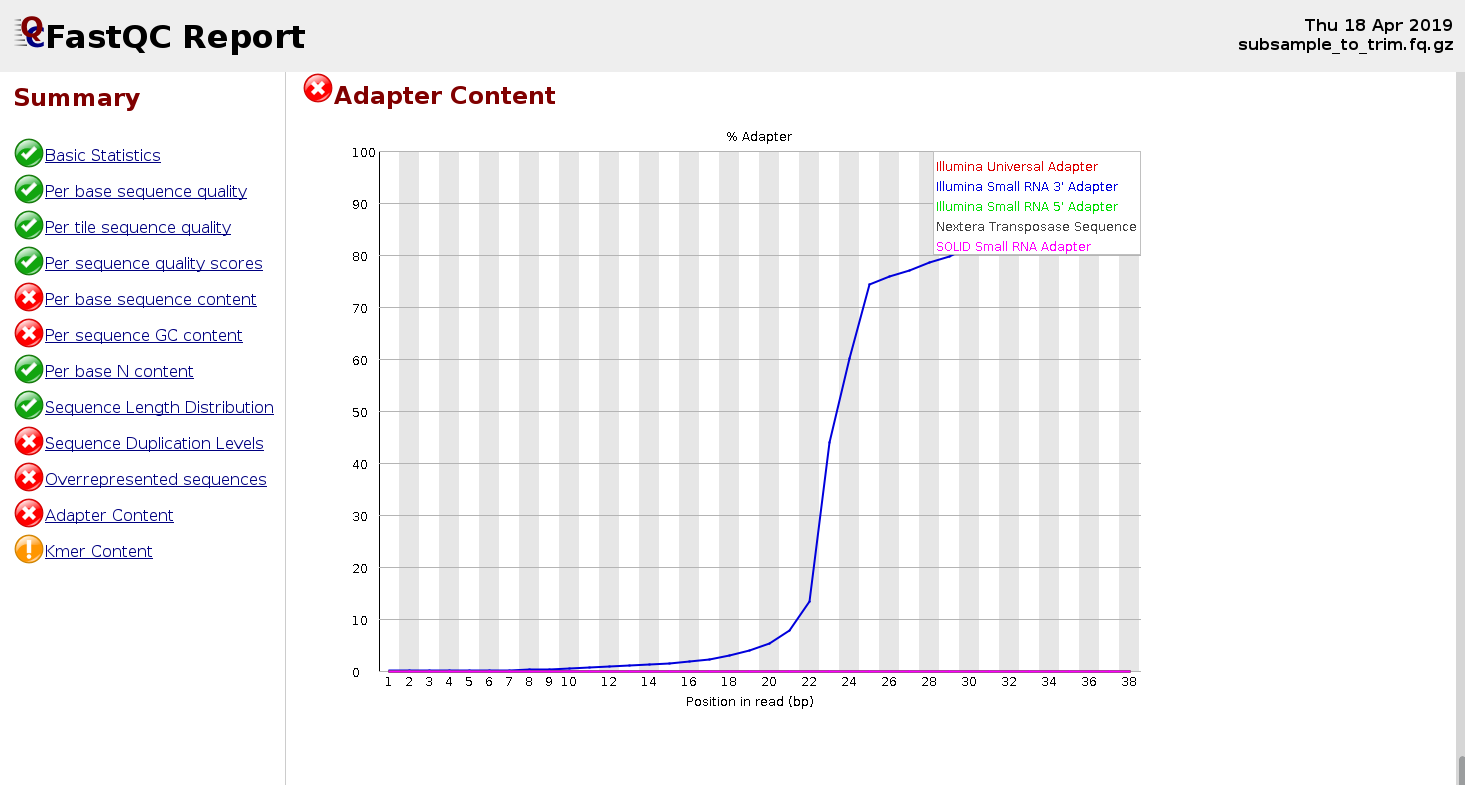
3. Adapter Content
Should be near 0% in well-prepared libraries
High adapter content indicates insufficient insert size or failed library prep
Adapters must be trimmed before alignment
This problem arises when the sequenced DNA fragment is shorter than the read length — the sequencer runs out of insert and reads into the adapter:
Ideal case (insert > read length):
  5'──────────────── INSERT ────────────────3'
  |←────── Read (150 bp) ──────→|

Problem case (insert < read length):
  5'──── INSERT ────3'
  |←──── Read ─────────────── ADAPTER →|
                   ↑
         Adapter sequence contaminates the read
4. Overrepresented Sequences
FastQC will BLAST-match overrepresented sequences
Common hits: TruSeq adapters, polyA tails, rRNA
Any unknown overrepresented sequence warrants investigation
Important — General rules do not apply to all applications
:class: important
The guides above apply to regular RNA-seq datasets. In other applications, these rules do not hold:
Small RNA-seq libraries: insert size is smaller and adapter content is expected to be higher (see example below).
Single-cell experiments: read 1 contains the cell barcode and UMI, so its GC content profile may be altered.
|
Figure 3: FastQC report for a small RNA-seq sample showing elevated adapter content |
Exercises I
The first part of this exercise is to download publicly available data from SRA, using the SRA toolkit. Below you can find the basic commands to use this tool:
# Download a single run (compressed .sra format)
prefetch SRR1234567

# Convert to FASTQ (single-end)
fasterq-dump SRR1234567 --outdir ./fastq/

# For paired-end data, split into R1 and R2
fasterq-dump SRR1234567 --split-files --outdir ./fastq/

# Compress the output (fasterq-dump does not gzip by default)
gzip ./fastq/SRR1234567.fastq
Now, download the data (accession number SRR36179215) using the SRA toolkit, run FastQC, and answer the questions below.
# Add command:
export RUN_SRA="singularity exec -e /home/training/sra-tools_3.3.0.sif"

cd ~/RNAseq_coursesCRG_2026/
mkdir exercise1_fastqc

# Download from SRA:
$RUN_SRA prefetch SRR36179215
$RUN_SRA fasterq-dump SRR36179215 --outdir ./exercise1/
gzip ./exercise1/SRR36179215.fastq

# Run FastQC
$RUN fastqc ./exercise1/SRR36179215.fastq.gz -o ./exercise1_fastqc/
firefox ./exercise1_fastqc/SRR36179215_fastqc.html &
Discussion questions:
Is this adapter content a sign of a failed experiment? Why or why not? Which type of dataset this might be?
Would you apply the same quality interpretation to a standard mRNA-seq dataset with this level of adapter content?
Note
Reads are shorter than what we can normally expect nowadays, because it is old data and also because it is convenient to run analyses faster for the course.
FastQ Screen
FastQ Screen screens reads to detect cross-species contamination or unexpected biological sequences. It is particularly useful for:
Detecting human contamination in non-human samples (and vice versa)
Identifying mycoplasma, PhiX, or E. coli contamination
Verifying the species of origin of a sample
The tool works by:
Taking a subsample (~100,000 reads by default, adjustable with
--subset)Aligning reads to each reference genome using Bowtie2
Reporting the percentage of reads mapping to each reference
Generating a stacked bar chart showing mapping distribution
Setting Up Databases
Warning
Do not run the following command in class — it will take too much time and resources.
# Download default databases
$RUN fastq_screen --get_genomes
This downloads 14 Bowtie2 indexes (model organisms and known contaminants):
Arabidopsis thaliana, Drosophila melanogaster, Escherichia coli
Homo sapiens, Mus musculus, Rattus norvegicus
Caenorhabditis elegans, Saccharomyces cerevisiae
Lambda, Mitochondria, PhiX, Adapters, Vectors, rRNA
Upon download, the FastQ_Screen_Genomes folder is created. You must provide a fastq_screen.conf configuration file with paths to the Bowtie2 binary and genome indices:
# This is a configuration file for fastq_screen

BOWTIE2 /usr/local/bin/bowtie2

## Human
DATABASE Human /path/to/FastQ_Screen_Genomes/Human/Homo_sapiens.GRCh38

## Mouse
DATABASE Mouse /path/to/FastQ_Screen_Genomes/Mouse/Mus_musculus.GRCm38

## E. coli
DATABASE Ecoli /path/to/FastQ_Screen_Genomes/E_coli/Ecoli

## PhiX
DATABASE PhiX /path/to/FastQ_Screen_Genomes/PhiX/phi_plus_SNPs

## Adapters
DATABASE Adapters /path/to/FastQ_Screen_Genomes/Adapters/contaminants
Running FastQ Screen
In the command below, you can see how to run fastq_screen in a single sample. IMPORTANT: due to time constrains, please do not run fastq_screen. If there is time, feel free to try it at the end of the hands-on session.
$RUN fastq_screen --conf FastQ_Screen_Genomes/fastq_screen.conf \
           sample.fq.gz \
           --outdir ~/RNAseq_coursesCRG_2026/raw_qc/
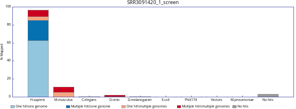
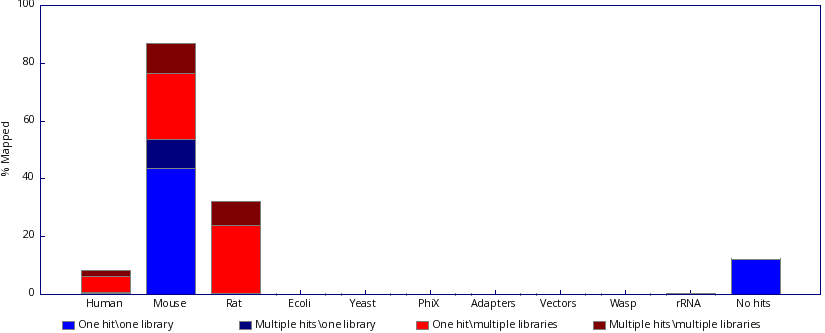
To view example results for SRR3091420_1_chr6.fastq.gz:
|
Figure 4: Fastq_screen results |
Output Files
sample_screen.html     # Visual HTML report with bar charts
sample_screen.txt      # Tab-delimited mapping statistics
Example _screen.txt output:
#Fastq_screen version: 0.15.3
Genome    #Reads_processed  #Unmapped  %Unmapped  #One_hit_one_genome  %One_hit  #Multiple_hits  %Multiple
Human     100000            95020      95.02      4830                 4.83      150             0.15
Mouse     100000            99780      99.78      180                  0.18      40              0.04
Ecoli     100000            99950      99.95      45                   0.05      5               0.00
PhiX      100000            100000     100.00     0                    0.00      0               0.00
Interpreting Results
FastQ Screen results require careful interpretation — context matters depending on which databases are in your config.
Column |
Meaning |
|---|---|
One hit, one genome |
Read maps uniquely to this genome only |
Multiple hits, one genome |
Read maps to this genome in multiple locations, but nowhere else |
One hit, multiple genomes |
Read maps uniquely within this genome, but also maps to other genomes |
Multiple hits, multiple genomes |
Read maps to multiple locations in this genome and in other genomes |
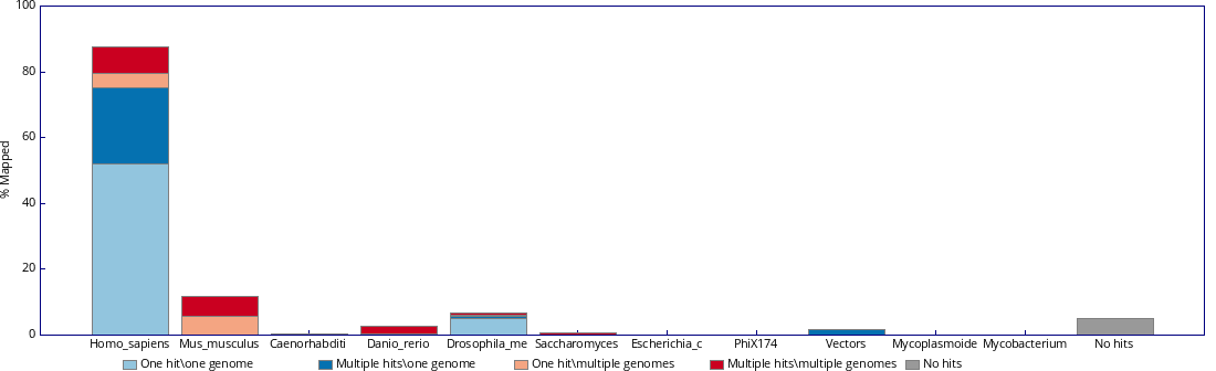
Exercises II
Check both fastq_screen outputs below. Inspect them carefully and justify which one reflects a contamination and which one is expected.
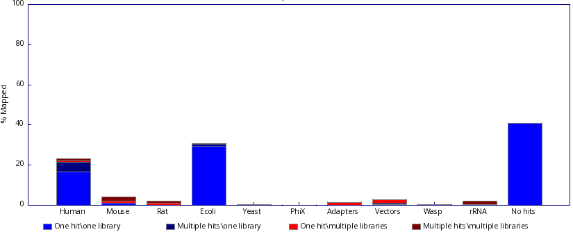
Inspect the fastq_screen output. What do you think is happening to the sample? Would you need to ask more information about it before reaching any conclusion?
|
Figure 7: Fastq screen output 3. |
Kraken2
Kraken2 performs k-mer based taxonomic classification of sequencing reads. Unlike FastQ Screen — which aligns to specific genomes — Kraken2 classifies reads against a broad taxonomic database, enabling detection of unexpected organisms at genus/species level.
Use cases:
Detecting microbial contamination in eukaryotic samples
Metagenomics community profiling
Validating microbial sequencing samples
Identifying viral contamination
How Kraken2 Works
Breaks each read into k-mers (default k=35)
Looks up each k-mer in a pre-built hash table of taxonomic assignments
Uses a lowest common ancestor (LCA) algorithm to assign a taxonomy
Reports classification at each taxonomic level (phylum → species)
Basic Usage
# Classify single-end reads
kraken2 \
    --db kraken2_db/ \
    --threads 8 \
    --report sample_kraken2_report.txt \
    --output sample_kraken2_output.txt \
    sample.fastq.gz

# Classify paired-end reads
kraken2 \
    --db kraken2_db/ \
    --threads 8 \
    --paired \
    --report sample_kraken2_report.txt \
    --output sample_kraken2_output.txt \
    sample_R1.fastq.gz sample_R2.fastq.gz
Understanding the Output
The report file (--report) follows this tab-delimited format:
% reads   # reads  # reads at taxon  rank  taxID   name
 78.50    78500    420               D     2       Bacteria
 15.20    15200    15200             S     9606    Homo sapiens
  5.10    5100     200               D     10239   Viruses
  1.20    1200     1200              U     0       unclassified
Column |
Description |
|---|---|
% reads |
Percentage of reads assigned to this taxon |
# reads |
Number of reads under this taxon (including children) |
# reads at taxon |
Reads assigned directly (not to children) |
rank |
D=Domain, P=Phylum, C=Class, O=Order, F=Family, G=Genus, S=Species |
taxID |
NCBI taxonomy ID |
name |
Taxonomic name |
Hands-on: Kraken2
# Uncompress the kraken2 database:
cd ~/RNAseq_indices/
tar -zxf minikraken2_v2_8GB_201904_UPDATE.tar.gz

# Classify single-end reads
cd ~/RNAseq_coursesCRG_2026

$RUN kraken2 \
    --db ~/RNAseq_indices/minikraken2_v2_8GB_201904_UPDATE \
    --output ~/RNAseq_coursesCRG_2026/raw_qc/SRR3091420_1_chr6_kraken_output.txt \
    --report ~/RNAseq_coursesCRG_2026/raw_qc/SRR3091420_1_chr6_kraken_report.txt \
    docs/data/reads/SRR3091420_1_chr6.fastq.gz
Exercises III:
Now, run Kraken2 for all of our samples and check the results. Are what do you expected? Do they match with those from fastq_screen?
# Go to the repository directory:
cd ~/RNAseq_coursesCRG_2026

# Run Kraken2 in all samples:

for fastq_file in ~/RNAseq_coursesCRG_2026/docs/data/reads/*.fastq.gz; do

    filename=$(basename "$fastq_file")

    # Strip extension(s): handles .fastq.gz, .fq.gz, .fastq, .fq
    sample_name="${filename%%.*}"

    # Set output and report names:
    output_path="$HOME/RNAseq_coursesCRG_2026/raw_qc/${sample_name}_kraken_output.txt"
    report_path="$HOME/RNAseq_coursesCRG_2026/raw_qc/${sample_name}_kraken_report.txt"


    $RUN kraken2 \
        --db ~/RNAseq_indices/minikraken2_v2_8GB_201904_UPDATE \
        --output $output_path \
        --report $report_path \
        $fastq_file
; done
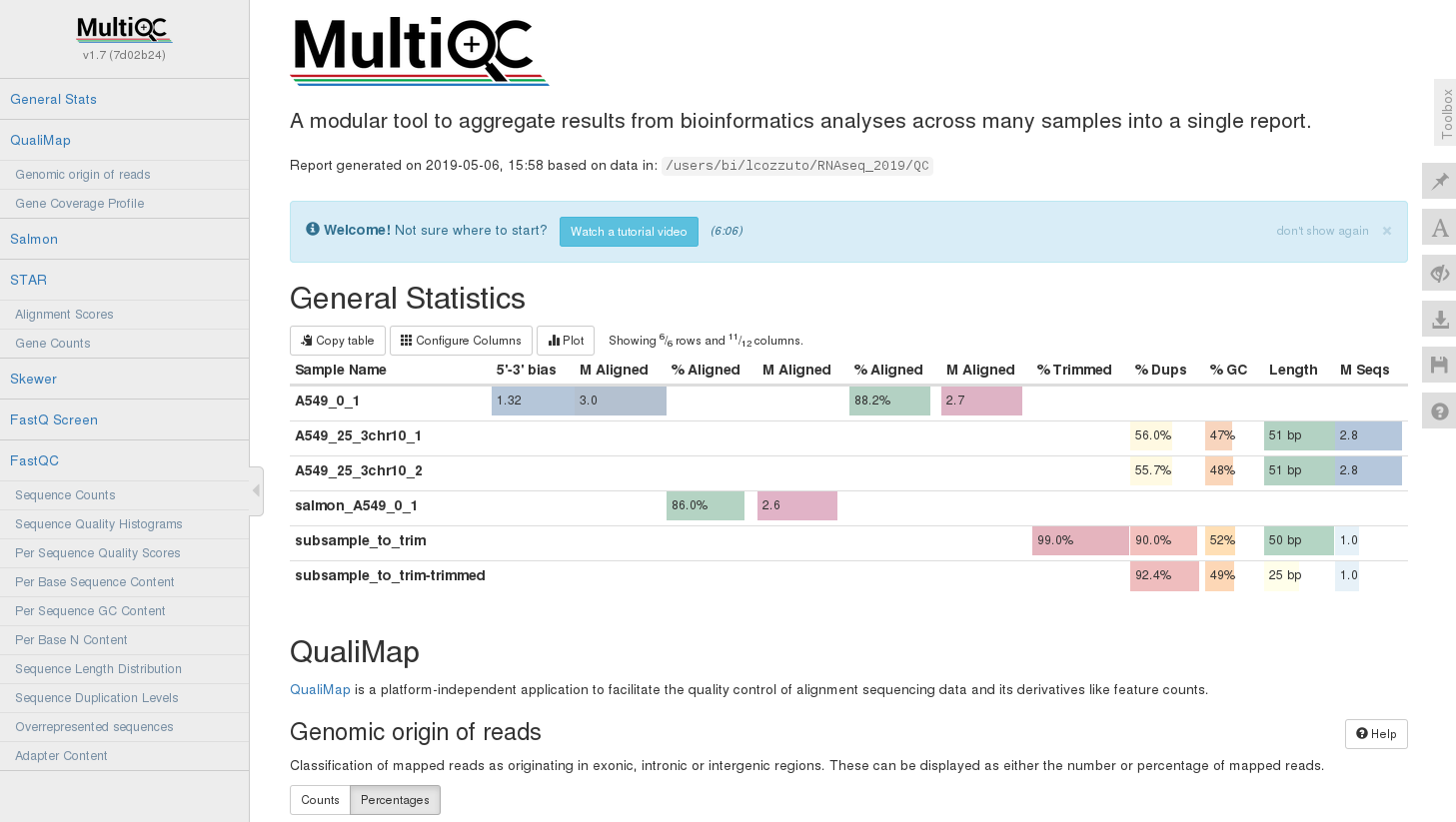
MultiQC
MultiQC aggregates QC reports from multiple tools and multiple samples into a single interactive HTML report. Instead of reviewing dozens of individual FastQC HTML files, MultiQC produces one unified dashboard.
Supported tools include: FastQC, FastQ Screen, Kraken2, Trimmomatic, STAR, HISAT2, Salmon, featureCounts, Picard, samtools, and many more.
Running MultiQC
cd ~/RNAseq_coursesCRG_2026/

# Create a folder for the MultiQC result
mkdir multiqc_report
cd ~/RNAseq_coursesCRG_2026/multiqc_report

# Link QC, trimming and mapping data
ln -s ~/RNAseq_coursesCRG_2026/raw_qc .

# Run MultiQC on the directory
$RUN multiqc .

# Visualize in browser
firefox multiqc_report.html &
|
Figure 8: Example of multiQC report (html). |
Read Pre-processing: adapter trimming and rRNA removal
After running raw QC, two issues commonly stand out in the MultiQC report that must be addressed before alignment:
Problem |
Consequence if not addressed |
|---|---|
Adapter sequences |
Misalignments, spurious variant calls, reduced mapping rate |
Low quality 3’ bases |
Increased error rate in alignments and assemblies |
rRNA reads |
Wasted sequencing depth; biased expression estimates |
Adapter Trimming
The Landscape of Tools
Several mature tools exist for adapter trimming and quality filtering. They share the same core goal but differ in speed, flexibility, and default behaviour.
Tool |
Language |
Strengths |
Typical Use Case |
|---|---|---|---|
Trimmomatic |
Java |
Highly configurable, widely used |
General Illumina trimming |
Cutadapt |
Python |
Precise adapter specification, great docs |
When adapters are known exactly |
TrimGalore |
Perl wrapper |
Auto-detects adapters, wraps Cutadapt + FastQC |
Most RNA-seq / WGS workflows |
fastp |
C++ |
Very fast, all-in-one QC + trim |
Large datasets, speed-critical |
BBDuk |
Java (BBTools) |
Flexible k-mer trimming, contaminant removal |
Complex filtering needs |
PRINSEQ |
Perl |
Broad filtering options including complexity |
Metagenomics, older workflows |
How Trimming Works
All tools follow the same general logic:
Step 1 — Adapter Sequence Matching: The tool is given (or detects) the known adapter sequence and searches for it within each read. When found, the adapter and everything 3’ of it is clipped. Most tools allow a configurable error rate to account for sequencing errors within the adapter.
Read:   ACGTACGTACGTACGT[AGATCGGAAGAGC...]
                         ↑ adapter match
Result: ACGTACGTACGTACGT
Step 2 — Quality-Based Trimming: Separately from adapter removal, tools can trim bases from the 3’ end below a Phred quality threshold. The most common algorithm is a sliding window approach: start from the 3’ end, calculate average quality in a window (e.g., 4 bp), remove it if below threshold, and repeat moving inward until the window passes.
Step 3 — Minimum Length Filtering: After trimming, reads that are too short to align reliably are discarded entirely (common threshold: 20–36 bp).
Important: how paired-end reads are handled
In paired-end mode, both reads of a pair must be handled together. If one read is discarded (too short after trimming), its partner must also be removed or placed in an “orphan” file to maintain pairing integrity — aligners require paired reads to be in the same order.
Trimming with TrimGalore
TrimGalore is a wrapper around Cutadapt and FastQC that adds automatic adapter detection, integrated FastQC re-running, and sensible defaults — making it the most practical choice for standard Illumina RNA-seq and WGS data.
# Single-end reads
trim_galore sample.fastq.gz

# Specify output directory and run FastQC on output
trim_galore --fastqc -o trimmed/ sample.fastq.gz
Key options:
trim_galore \
    --quality 20 \              # Trim 3' bases below Q20 (default: 20)
    --length 36 \               # Discard reads shorter than 36 bp after trimming
    --stringency 3 \            # Minimum adapter overlap (default 1; increase to avoid over-trimming)
    --fastqc \                  # Run FastQC on output
    --cores 4 \                 # Parallel processing
    -o trimmed_output/ \
    sample.fastq.gz
Specifying adapters manually:
# Illumina TruSeq adapter (most common for single-end)
trim_galore \
    --adapter AGATCGGAAGAGCACACGTCTGAACTCCAGTCA \
    sample.fastq.gz

# Nextera adapter
trim_galore --nextera sample.fastq.gz

# Small RNA (miRNA) adapter
trim_galore --small_rna sample.fastq.gz
Hands-on: Trim Galore
cd ~/RNAseq_coursesCRG_2026/

# Create a folder for the trimmed data:
mkdir trimmed_data

$RUN trim_galore \
    --quality 20 \
    -o trimmed_data/ \
    ~/RNAseq_coursesCRG_2026/docs/data/reads/SRR3091420_1_chr6.fastq.gz
Output files:
trimmed_data/
├── SRR3091420_1_chr6_trimmed.fq.gz                      # Trimmed reads
└── SRR3091420_1_chr6.fastq.gz_trimming_report.txt       # Trimming stats
Reading the trimming report:
Total reads processed:                 835,169
Reads with adapters:                   277,510 (33.2%)
Reads written (passing filters):       835,169 (100.0%)

Total basepairs processed:    40,923,281 bp
Quality-trimmed:                       0 bp (0.0%)
Total written (filtered):     40,540,114 bp (99.1%)
Key numbers to check:
Reads with adapters: confirms the adapter contamination seen in FastQC
Reads written (passing filters): should remain high (>95%); low values suggest aggressive trimming or very short inserts
Exercises IV
Adapt the code provided in exercise III (Kraken2) and, together with the trim-galore code above, modify it to run trimming in all of our samples. Afterwards, check the results and see if all samples behave similarly.
Solution
# Go to the repository directory:
cd ~/RNAseq_coursesCRG_2026

# Run Kraken2 in all samples:

for fastq_file in ~/RNAseq_coursesCRG_2026/docs/data/reads/*.fastq.gz; do

    $RUN trim_galore \
    --quality 20 \
    --fastqc \
    -o trimmed_data/ \
    "$fastq_file"

done
rRNA Removal with RiboDetector
Even after trimming, RNA-seq libraries often retain a proportion of ribosomal RNA reads from incomplete ribo-depletion (e.g., RiboZero, RNase H) or polyA selection inefficiency. These reads:
Consume sequencing depth without contributing to gene expression estimates
Inflate total read counts relative to informative mRNA reads
RiboDetector is a deep learning-based tool that accurately identifies and removes rRNA reads without relying on a reference database. It uses a neural network trained on a broad set of rRNA sequences from bacteria, archaea, and eukaryotes, enabling robust detection even for divergent or novel rRNA sequences.
Advantages over alignment-based tools:
No reference database download or maintenance required
Faster and more memory-efficient than alignment-based approaches
Handles partial rRNA matches and divergent sequences well
GPU acceleration available for large datasets
Basic Usage
# Single-end reads
ribodetector_cpu \
    -t 8 \
    -l 49 \
    -i sample_R1_trimmed.fq.gz \
    -e rrna \
    --rrna rrna.fq.gz \
    -o nonrrna.fq.gz

# Paired-end reads
ribodetector_cpu \
    -t 8 \
    -l 49 \
    -i sample_R1_trimmed.fq.gz sample_R2_trimmed.fq.gz \
    -e rrna \
    --rrna rrna_R1.fq.gz rrna_R2.fq.gz \
    -o nonrrna_R1.fq.gz nonrrna_R2.fq.gz
Key Parameters
Parameter |
Description |
|---|---|
|
Number of threads |
|
Read length (bp) — should match your actual read length after trimming |
|
Input FASTQ file(s) |
|
Ensure rRNA reads are written to the |
|
Output file for detected rRNA reads |
|
Output file for non-rRNA reads (use downstream) |
|
Number of reads processed per batch (default: 256; increase for speed if RAM allows) |
Hands-on: Ribodetector
cd ~/RNAseq_coursesCRG_2026/

# Create a folder for the trimmed data:
mkdir ribodetector
cd ribodetector

# Ribodetector does not give us a % of rRNA reads per se, so we will have to calculate it apart of running the tool:

tot=$(( $(zcat ~/RNAseq_coursesCRG_2026/trimmed_data/SRR3091420_1_chr6_trimmed.fq.gz | wc -l) / 4 ))

length=` zcat ~/RNAseq_coursesCRG_2026/trimmed_data/SRR3091420_1_chr6_trimmed.fq.gz | awk '{num++}{if(num%4==2) {seq++; len+=length(\$0)}}END{print int(len/seq)}' `

$RUN ribodetector_cpu \
-l $length \
-o SRR3091420_1_chr6_nonrrna.fq.gz -e rrna -r SRR3091420_1_chr6_rrna.fq.gz \
-i ~/RNAseq_coursesCRG_2026/trimmed_data/SRR3091420_1_chr6_trimmed.fq.gz

awk -v tot=$tot \
    '{num++} END{print id" "num/4/tot*100}' \
    <(zcat SRR3091420_1_chr6_rrna.fq.gz) > SRR3091420_1_chr6_trimmed_rna_perc.txt
Output Files
ribodetector_output/
├── SRR3091420_1_chr6_rrna.fq.gz       # rRNA reads (removed from analysis)
└── SRR3091420_1_chr6_nonrrna.fq.gz    # Clean reads
└── SRR3091420_1_chr6_trimmed_rna_perc.txt # Percentage of %rRNA reads
Interpreting the Output
A rRNA percentage of 1–10% is typical for well-depleted libraries. Values >20–30% suggest ribo-depletion failure and should be flagged, though the reads can still be usable after removal.
MultiQC - Post-Processing QC
Now, once we have finished the preprocessing, it is time to colapse all results into a multiQC report, which will contain pre- and post-trimming results, enabling direct side-by-side comparison.
Hands-on: multiQC
# Go to the working directory:
cd ~/RNAseq_coursesCRG_2026/multiqc_report

# Link trimming data:
ln -s ~/RNAseq_coursesCRG_2026/trimmed_data .

# Run multiQC:
$RUN multiqc raw_qc/ trimmed_data/ -n 'Raw_trimmed_qc' -d --dirs-depth 1 --force

firefox ~/RNAseq_coursesCRG_2026/multiqc_report/Raw_trimmed_qc.html &
Final Exercise
The file ~/RNAseq_coursesCRG_2026/docs/data/reads/example2_reads.fq.gz contains a set of single-end reads from an unknown sample. Apply the full pre-processing pipeline we covered in this session:
Run FastQC on the raw reads and inspect the HTML report.
Run FastQ Screen to check for cross-species contamination.
Run Kraken2 to perform taxonomic classification.
Run TrimGalore to remove adapters and low-quality bases.
Run RiboDetector to remove rRNA reads from the trimmed output.
Run FastQC again on both the processed reads.
Aggregate all results with MultiQC and compare the pre- and post-processing reports.
Once you have inspected all the outputs, consider the following questions:
Which results from the quality control are unexpected for a standard RNA-seq dataset? Describe what you observe and why it deviates from what would normally be considered “good” quality.
Can you think of a specific sequencing application where those results would actually be expected and perfectly normal? Explain your reasoning.
Further Reading
Documentation
FastQC: https://www.bioinformatics.babraham.ac.uk/projects/fastqc/
FastQ Screen: https://www.bioinformatics.babraham.ac.uk/projects/fastq_screen/
MultiQC: https://multiqc.info/docs/ — Module list: https://multiqc.info/modules/
TrimGalore: https://www.bioinformatics.babraham.ac.uk/projects/trim_galore/ — User Guide: https://github.com/FelixKrueger/TrimGalore/blob/master/Docs/Trim_Galore_User_Guide.md
Cutadapt: https://cutadapt.readthedocs.io/
RiboDetector: https://github.com/hzi-bifo/RiboDetector
Key Articles
Andrews, S. (2010). FastQC: A Quality Control Tool for High Throughput Sequence Data.
Wingett, S. & Andrews, S. (2018). FastQ Screen: A tool for multi-genome mapping and quality control. F1000Research, 7, 1338. https://doi.org/10.12688/f1000research.15931.2
Wood, D.E. et al. (2019). Improved metagenomic analysis with Kraken 2. Genome Biology, 20, 257. https://doi.org/10.1186/s13059-019-1891-0
Ewels, P. et al. (2016). MultiQC: Summarize analysis results for multiple tools and samples in a single report. Bioinformatics, 32(19), 3047–3048. https://doi.org/10.1093/bioinformatics/btw354
Martin, M. (2011). Cutadapt removes adapter sequences from high-throughput sequencing reads. EMBnet.journal, 17(1), 10–12. https://doi.org/10.14806/ej.17.1.200
Bolger, A.M. et al. (2014). Trimmomatic: a flexible trimmer for Illumina sequence data. Bioinformatics, 30(15), 2114–2120. https://doi.org/10.1093/bioinformatics/btu170
Deng, Z. et al. (2022). RiboDetector: accurate and rapid RiboRNA sequences detector based on deep learning. Nucleic Acids Research, 50(10), e60. https://doi.org/10.1093/nar/gkac112