Functional analysis

First, get the files from the undifferentiated only DESeq2 analysis (in case we did not have time to do it):

# get file
wget https://public-docs.crg.es/biocore/projects/training/PHINDaccess2020/undiff.tar.gz

# extract archive
tar -xvzf undiff.tar.gz

# remove archive
rm undiff.tar.gz

Data bases

Gene Ontology

The Gene Ontology (GO) describes our knowledge of the biological domain with respect to three aspects:

GO domains / root terms	Description
Molecular Function	Molecular-level activities performed by gene products. e.g. catalysis, binding.
Biological Process	Larger processes accomplished by multiple molecular activities. e.g. apoptosis, DNA repair.
Cellular Component	The locations where a gene product performs a function. e.g. cell membrane, ribosome.

Example of GO annotation: the gene product “cytochrome c” can be described by the molecular function oxidoreductase activity, the biological process oxidative phosphorylation, and the cellular component mitochondrial matrix.

The structure of GO can be described as a graph: each GO term is a node, each edge represents the relationships between the nodes. For example:

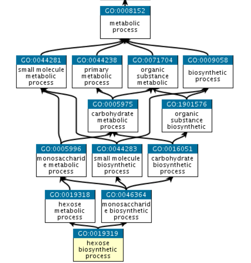
GO:0019319 (hexose biosynthetic process) is part of GO:0019318 (hexose metabolic process) and also part of GO:0046364 (monosaccharide biosynthetic process). They all share common parent nodes, for example GO:0008152 (metabolic process), and eventually a root node that is here biological process.

KEGG pathways

The Kyoto Encyclopedia of Genes and Genomes (KEGG) is a database for understanding high-level functions and utilities of the biological system.

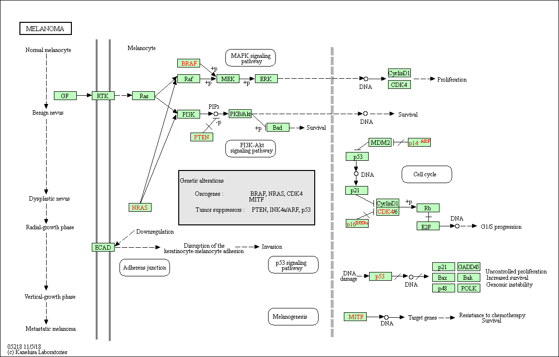
It provides comprehensible manually-drawn pathways representing biological processes or disease-specific pathways.
Example of the Homo sapiens melanoma pathway:

Molecular Signatures Database (MSigDB)

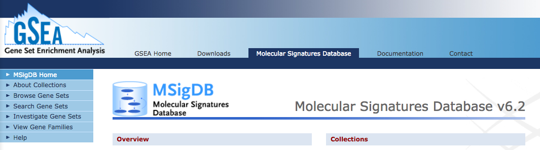
The Molecular Signatures Database (MSigDB) is a collection of 17810 annotated gene sets (as of May 2019) created to be used with the GSEA software (but not only).

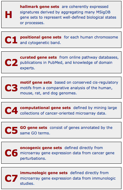
It is divided into 8 major collections (that include the previously described Gene Ontologies and KEGG pathways):

Enrichment analysis based on gene selection

Tools based on a user-selection of genes usually require 2 inputs:

• Gene Universe: in our example: all genes used in our analysis (after filtering out low counts in our case).
• List of genes selected from the universe: our selection of genes, give the criteria we previously used: padj < 0.05.

They are often based on the Hypergeometric test or on the Fisher’s exact test. You can have a look at this page for some explanation of both tests.

Let’s prepare this list from the file we saved before:

cd ~/rnaseq_course/functional_analysis

# The gene symbol is in the 12th column
cut -f 12 ~/rnaseq_course/differential_expression/undiff/deseq2_selection_padj005_undiff.txt | sed '1d' > deseq2_selection_padj005_symbols.txt

enrichR

EnrichR is a gene-list enrichment tool developped at the Icahn Schoold of Medicine (Mount Sinai).

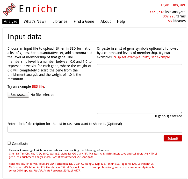
It does not require the input of a gene universe: only a selection of genes or a BED file.

The default EnrichR interface works for Homo sapiens and Mus musculus.
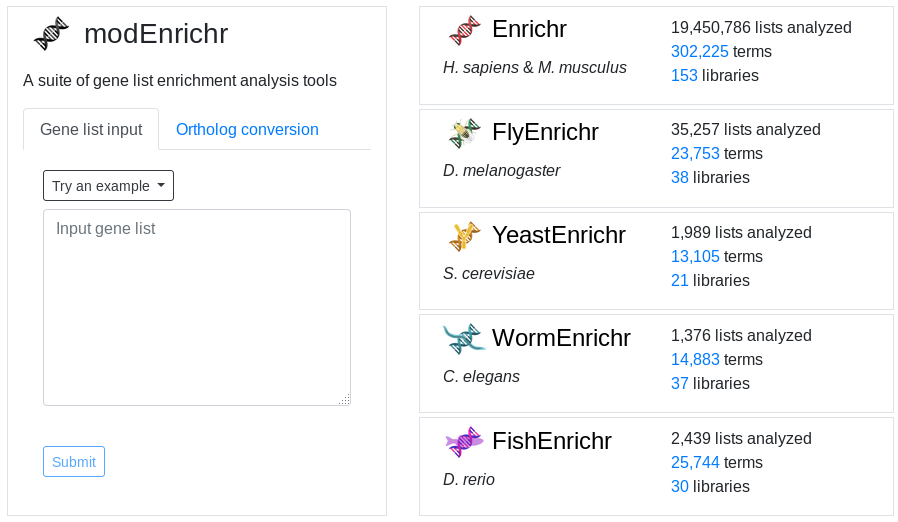
However, EnrichR also provides a set of tools for ortholog conversion and enrichment analysis of more organisms:

In the main page, paste our list of selected gene symbols (deseq2_selection_padj005_symbols.txt) and Submit !

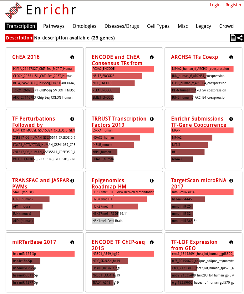
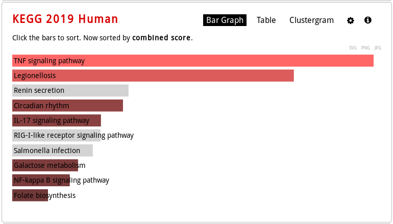
KEGG Human pathway bar graph vizualization:

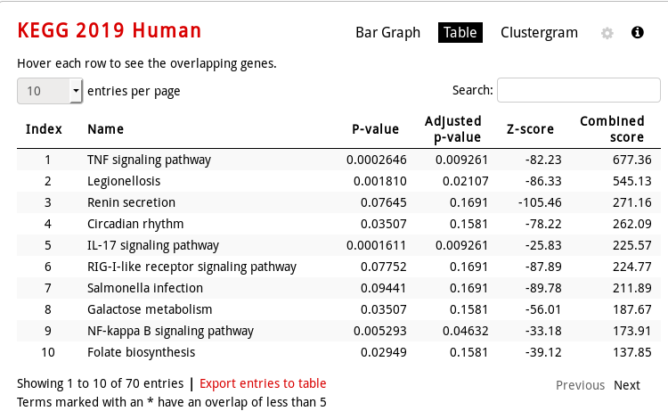
KEGG Human pathway table vizualization:

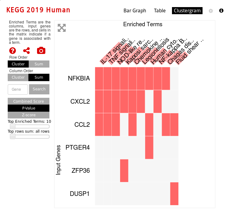
KEGG Human pathway clustergram vizualization:

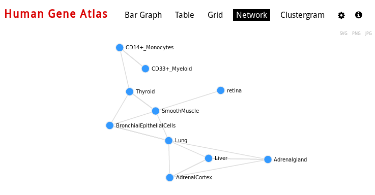
For Cell Types, you can also visualize networks, for example Human gene Atlas:

You can also export some graphs as PNG, JPEG or SVG.

GO / Panther tool

The main page of GO provides a tool to test the enrichment of gene ontologies or Panther/Reactome pathways in pre-selected gene lists.
The tool needs a selection of differentially expressed genes (supported IDs are: gene symbols, ENSEMBL IDs, HUGO IDs, UniGene, ..) and a gene universe.

Prepare files using s time the ENSEMBL IDs:

cd ~/rnaseq_course/functional_analysis

# Extract all gene IDs used in our analysis
cut -f 1 ~/rnaseq_course/differential_expression/undiff/normalized_counts_log2_star_undiff.txt | sed '1d' > deseq2_UNIVERSE_ENSEMBL.txt

# Extract significant gene symbols only
cut -f 1 ~/rnaseq_course/differential_expression/undiff/deseq2_selection_padj005_undiff.txt | sed '1d' > deseq2_selection_padj005_ENSEMBL.txt

Paste our selection, and select biological process and Homo sapiens:

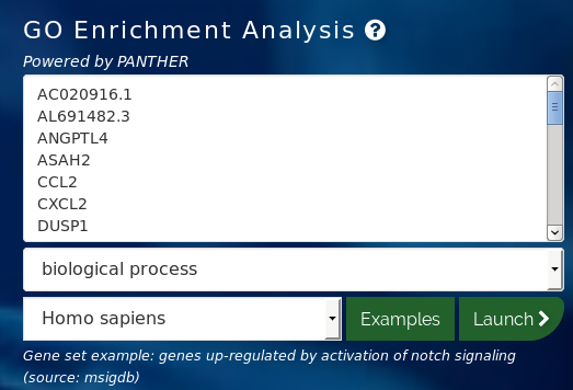
Launch !

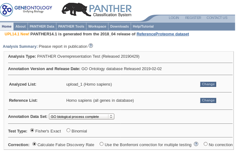
Analyzed List is what we just uploaded (deseq2_selection_padj005_ENSEMBL.txt).
In Reference List, we need to upload a file containg the universe (deseq2_UNIVERSE_ENSEMBL.txt): Change -> Browse -> (select deseq2_UNIVERSE_ENSEMBL.txt) -> Upload list

• Launch analysis
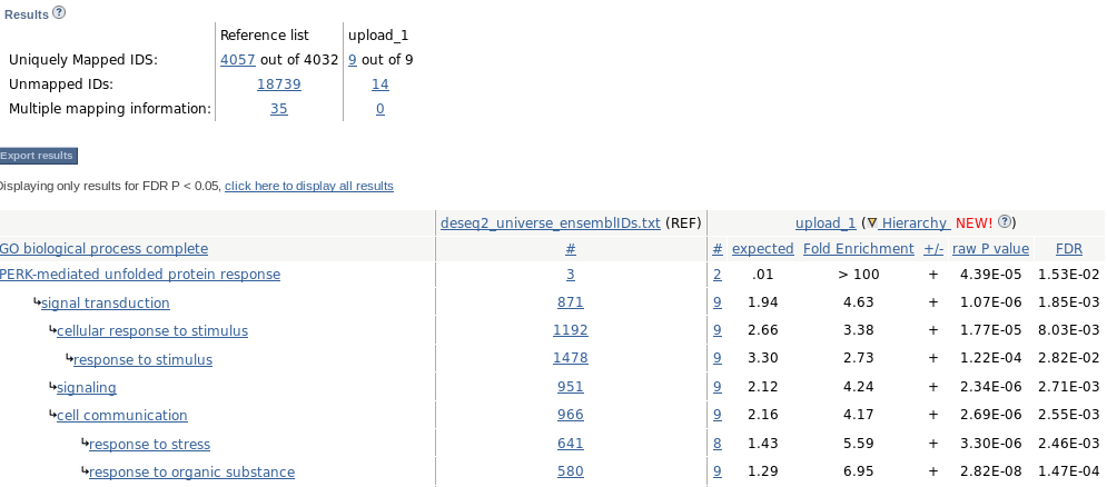
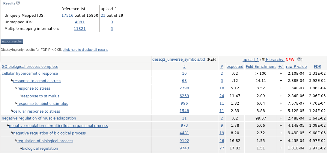
• Try the same analysis using the gene symbols instead of ENSEMBL IDs

  # Get universe with gene symbols (we already have the gene selection in deseq2_selection_padj005_symbol.txt
  cut -f11 ~/rnaseq_course/differential_expression/undiff/normalized_counts_log2_star_undiff.txt | sed '1d' > deseq2_UNIVERSE_symbols.txt
  

• Launch !

with R: GOstats

In RStudio, load the “GOstats” package

setwd("~/rnaseq_course/functional_analysis")

library("GOstats")

Read in differentially expressed genes

de_select <- read.table("deseq2_selection_padj005_ENSEMBL.txt", header=T, as.is=T, sep="\t")

The gene universe can be the list of genes after filtering for low counts: we prepared it already: deseq2_UNIVERSE_ENSEMBL.txt

de_univ <- read.table("deseq2_UNIVERSE_ENSEMBL.txt", header=T, as.is=T, sep="\t")

GOstats works only with Entrez IDs: we can get them with the biomaRt package, as we did for the differential expression analysis.

library(biomaRt)


# load database
mart <- useMart(biomart="ENSEMBL_MART_ENSEMBL", host="mar2017.archive.ensembl.org", path="/biomart/martservice", dataset="hsapiens_gene_ensembl")

# ENSEMBL IDs for differentially expressed genes
ids <- de_select

# get Entrez IDs
entrez <- getBM(attributes=c('entrezgene', 'ensembl_gene_id'), filters ='ensembl_gene_id', values = ids, mart = mart)

# get Entrez IDs for the universe
ids_univ <- de_univ
entrez_univ <- getBM(attributes=c('entrezgene', 'ensembl_gene_id'), filters ='ensembl_gene_id', values = ids_univ, mart = mart)

As biomaRt is causing trouble, you can get the files the following way

download.file("https://public-docs.crg.es/biocore/projects/training/PHINDaccess2020/deseq2_UNIVERSE_entrez.txt")
download.file("https://public-docs.crg.es/biocore/projects/training/PHINDaccess2020/deseq2_selection_padj005_entrez.txt")

entrez <- scan("deseq2_selection_padj005_entrez.txt")
entrez_univ <- scan("deseq2_UNIVERSE_entrez.txt")

We can proceed with the hypergeometric test (enrichment) for the Biological Process ontologies:

# install annotation package
BiocManager::install("org.Hs.eg.db")

# Set p-value cutoff
hgCutoff <- 0.001

# Set parameters
params <- new("GOHyperGParams",
	geneIds=na.omit(unique(entrez)),
	universeGeneIds=na.omit(unique(entrez_univ)),
	ontology="BP",
	annotation="org.Hs.eg",
	pvalueCutoff=hgCutoff,
	conditional=FALSE,
	testDirection="over")

# Run enrichment test
hgOver <- hyperGTest(params)

# Get a summary table
df <- summary(hgOver)

GOBPID	Pvalue	OddsRatio	ExpCounts	Counts	Size	Term
GO:0016477	4.322880e-05	3.594820	5.82993675	17	1098	cell migration
GO:0010884	7.630680e-05	45.181065	0.08495354	3	16	positive regulation of lipid storage
GO:0097755	8.408726e-05	19.842188	0.23362224	4	44	positive regulation of blood vessel diameter
GO:0060485	9.996919e-05	7.305817	1.08315765	7	204	mesenchyme development
GO:0035150	1.250790e-04	11.541689	0.48848286	5	92	regulation of tube size
GO:0035296	1.250790e-04	11.541689	0.48848286	5	92	regulation of tube diameter

GOstats also provides an HTML report:

# Produce HTML report
htmlReport(hgOver, file="GOstats_BP.html")

We can open the report in a web browser.

With R: KEGGprofile

Load KEGGprofile package:

library(KEGGprofile)

KEGGprofile also works with Entrez ID (we got them for the GOstats analysis).

# KEGG pathway enrichment
KEGGresult <- find_enriched_pathway(na.omit(unique(entrez$entrezgene)), 
	returned_genenumber=10, 
	species='hsa', 
	download_latest = TRUE)

# Format file file
kegg_final <- data.frame(KEGGresult$stastic, 
	genes_entrezid=unlist(lapply(KEGGresult$detail, function(x)paste(x, collapse=",")), use.names=F), 
	stringsAsFactors=F)

# Write table to file
write.table(kegg_final, "KEGGprofile_results.txt", sep="\t", row.names=F, col.names=T, quote=F)

Results table:

Pathway_Name	Gene_Found	Gene_Pathway	Percentage	pvalue	pvalueAdj
Metabolic pathways	88	1489	0.06	4.644397e-08	1.565162e-05
Cytokine-cytokine receptor interaction	26	294	0.09	3.187192e-05	3.580279e-03
Viral protein interaction with cytokine and cytokine receptor	12	100	0.12	1.671507e-04	8.047114e-03
NF-kappa B signaling pathway	10	102	0.10	2.490180e-03	3.356763e-02
Mitophagy - animal	11	65	0.17	8.801457e-06	1.483046e-03
C-type lectin receptor signaling pathway	10	104	0.10	2.898658e-03	3.757106e-02

Enrichment based on ranked lists of genes using GSEA

GSEA (Gene Set Enrichment Analysis)

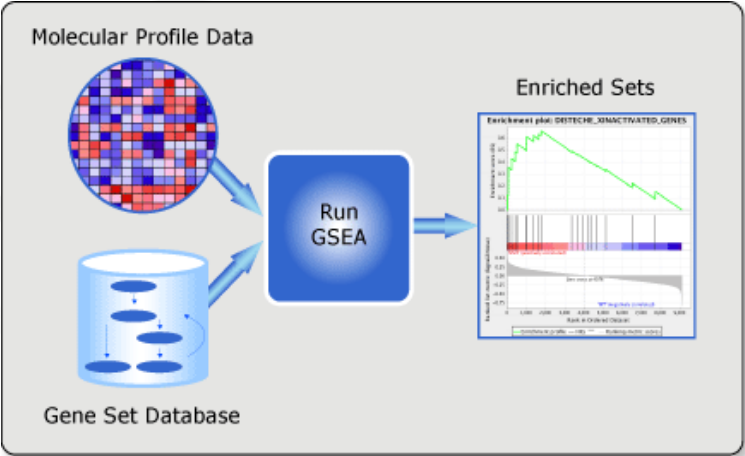
GSEA is available as a Java-based tool.

Algorithm

GSEA doesn’t require a threshold: the whole set of genes is considered.

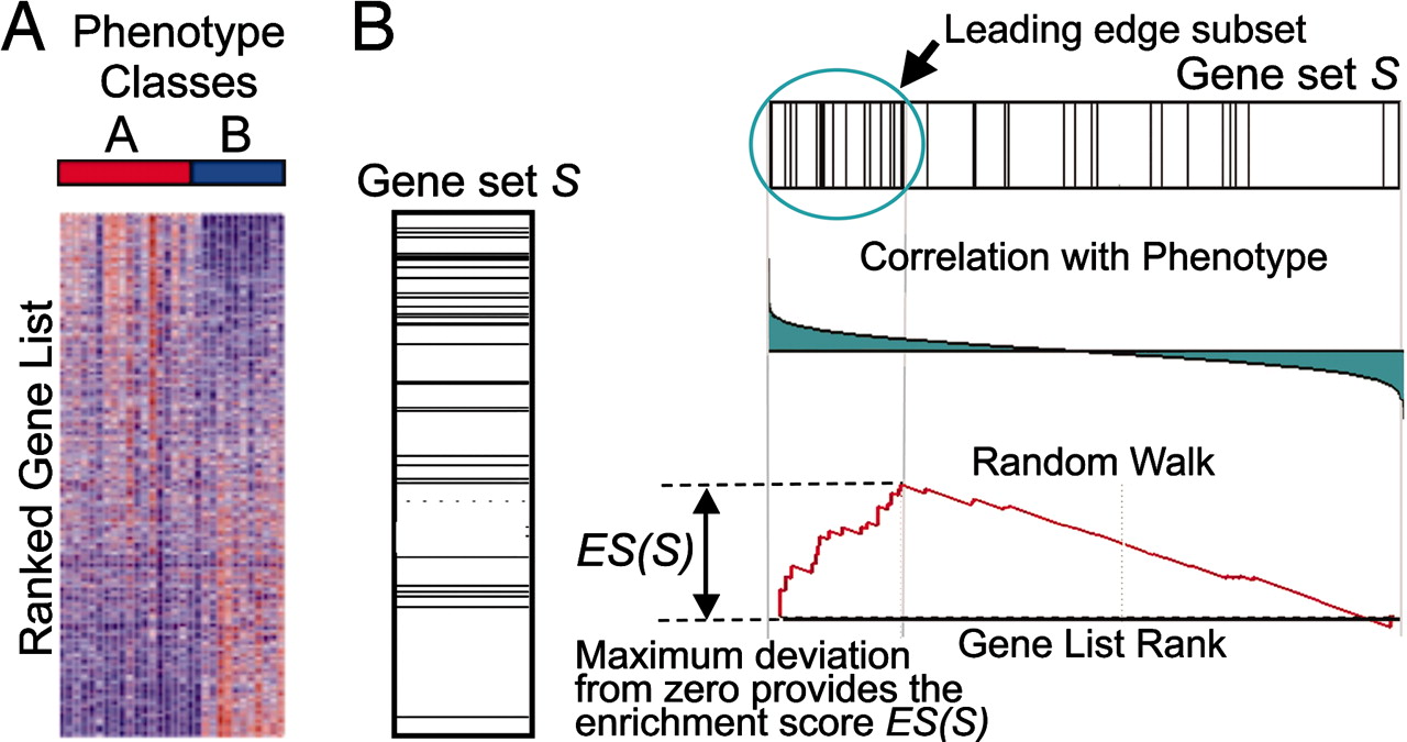
GSEA checks whether a particular gene set (for example, a gene ontology) is randomly distributed across a list of ranked genes.
The algorithm consists of 3 key elements:

1. Calculation of the Enrichment Score The Enrichment Score (ES) reflects the degree to which a gene set is overrepresented at the extremes (top or bottom) of the entire ranked gene list.
2. Estimation of Significance Level of ES The statistical significant (nominal p-value) of the Enrichment Score (ES) is estimated by using an empirical phenotype-based permutation test procedure. The Normalized Enrichment Score (NES) is obtained by normalizing the ES for each gene set to account for the size of the set.
3. Adjustment for Multiple Hypothesis Testing Calculation of the FDR ti control the proportion of falses positives.

See the GSEA Paper for more details on the algorithm.

The main GSEA algorithm requires 3 inputs:

• Gene expression data
• Phenotype labels
• Gene sets

Gene expression data in TXT format

The input should be normalized read counts filtered out for low counts (-> we created it in the DESeq2 tutorial -> normalized_counts.txt !).
The first column contains the gene ID (HUGO symbols for Homo sapiens).
The second column contains any description or symbol, and will be ignoreed by the algorithm.
The remaining columns contains normalized expressions: one column per sample.

NAME	DESCRIPTION	5p4_25c	5p4_27c	5p4_28c	5p4_29c	5p4_30c	5p4_31cfoxc1	…
DKK1	NA	0	0	0	0	0	0	…
HGT	NA	0	0	0	0	0	0	…

Exercise
Adjust the file normalized_counts_log2_star.txt so the first column is the gene symbol, the second is the gene ID (or anything else), and the remaining ones are the expression columns. You can save that new file as gsea_normalized_counts.txt.

cd ~/rnaseq_course/functional_analysis

awk -F "\t" 'BEGIN{OFS="\t"}{print $16,$1,$2,$3,$4,$5,$6,$7,$8,$9,$10,$11}' ~/rnaseq_course/differential_expression/normalized_counts_log2_star.txt > gsea_normalized_counts.txt

Phenotype labels in CLS format

A phenotype label file defines phenotype labels (experimental groups) and assigns those labels to the samples in the corresponding expression data file.

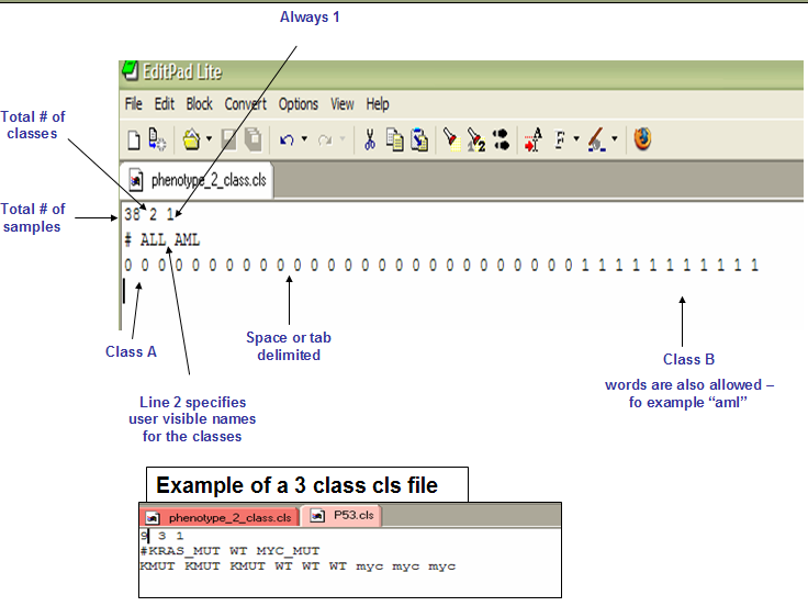
Let’s create it for our experiment:

10	2	1
#	WT	KO
WT	WT	WT	WT	WT	KO	KO	KO	KO	KO

NOTE: the first label used is assigned to the first class named on the second line; the second unique label is assigned to the second class named; and so on.
So the phenotype file could also be:

10	2	1
#	WT	KO
0	0	0	0	0	1	1	1	1	1

The first label WT in the second line is associated to the first label 0 on the third line.

Exercise
Create the phenotype labels file and save it as gsea_phenotypes.cls.

Download and run GSEA

Download Java application:

Enter the registration page, enter your email and organization, then to download page, enter your Email and login:
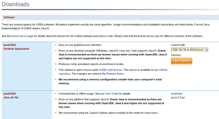
Click on download gsea-3.0.jar link and save file locally to your home directory.

Launch the GSEA application

GSEA is Java-based. Launch it from a terminal window:

$RUN java -Xmx1024m -jar gsea-3.0.jar

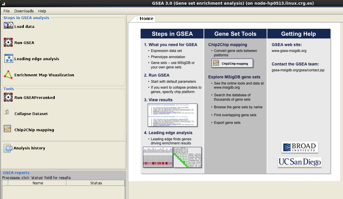
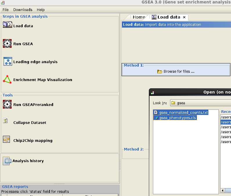
In Steps in GSEA analysis (upper left corner):

• Go to Load data: select gsea_normalized_counts.txt and gsea_phenotypes.cls and load.

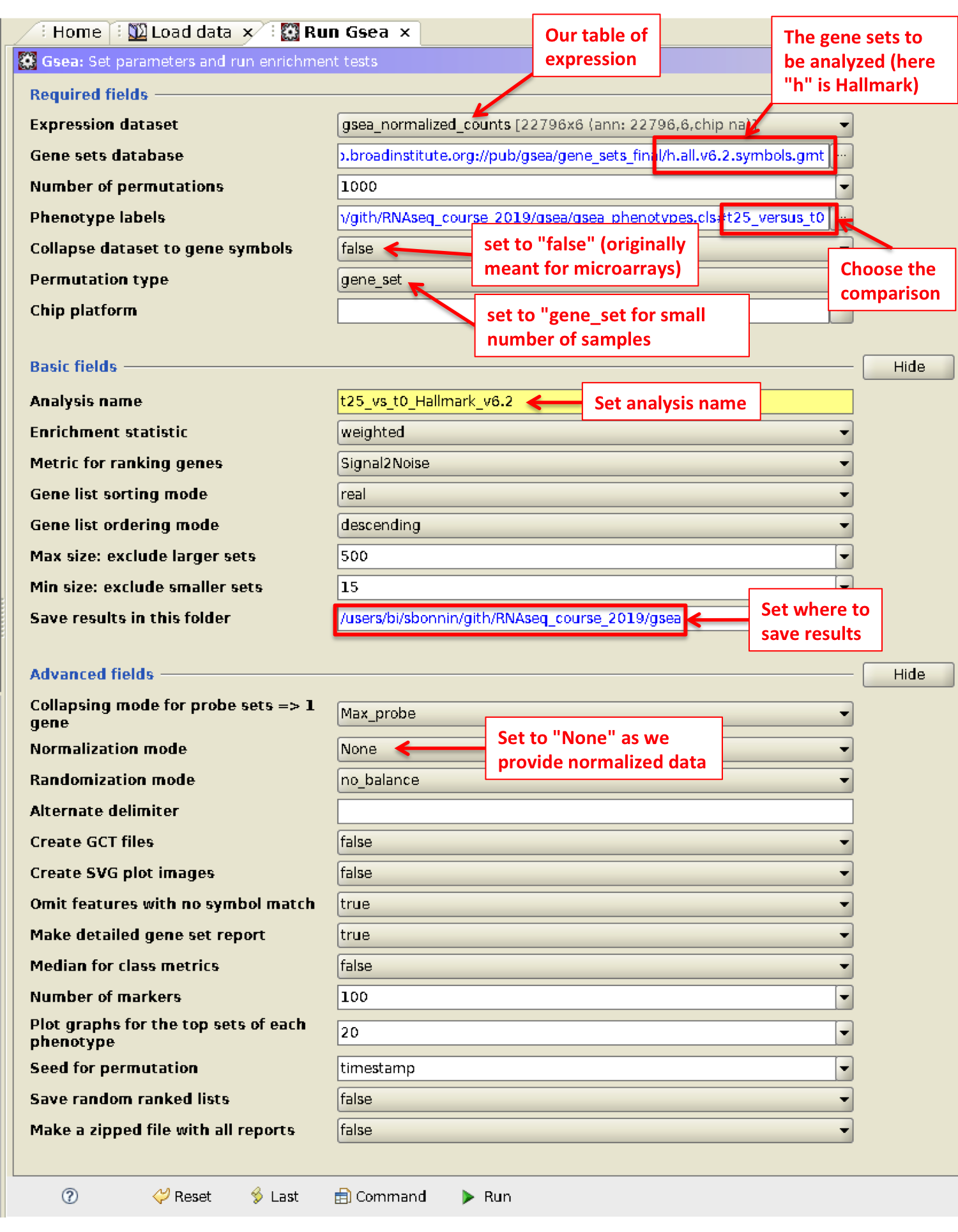
• Go to Run GSEA

• Results: index.html

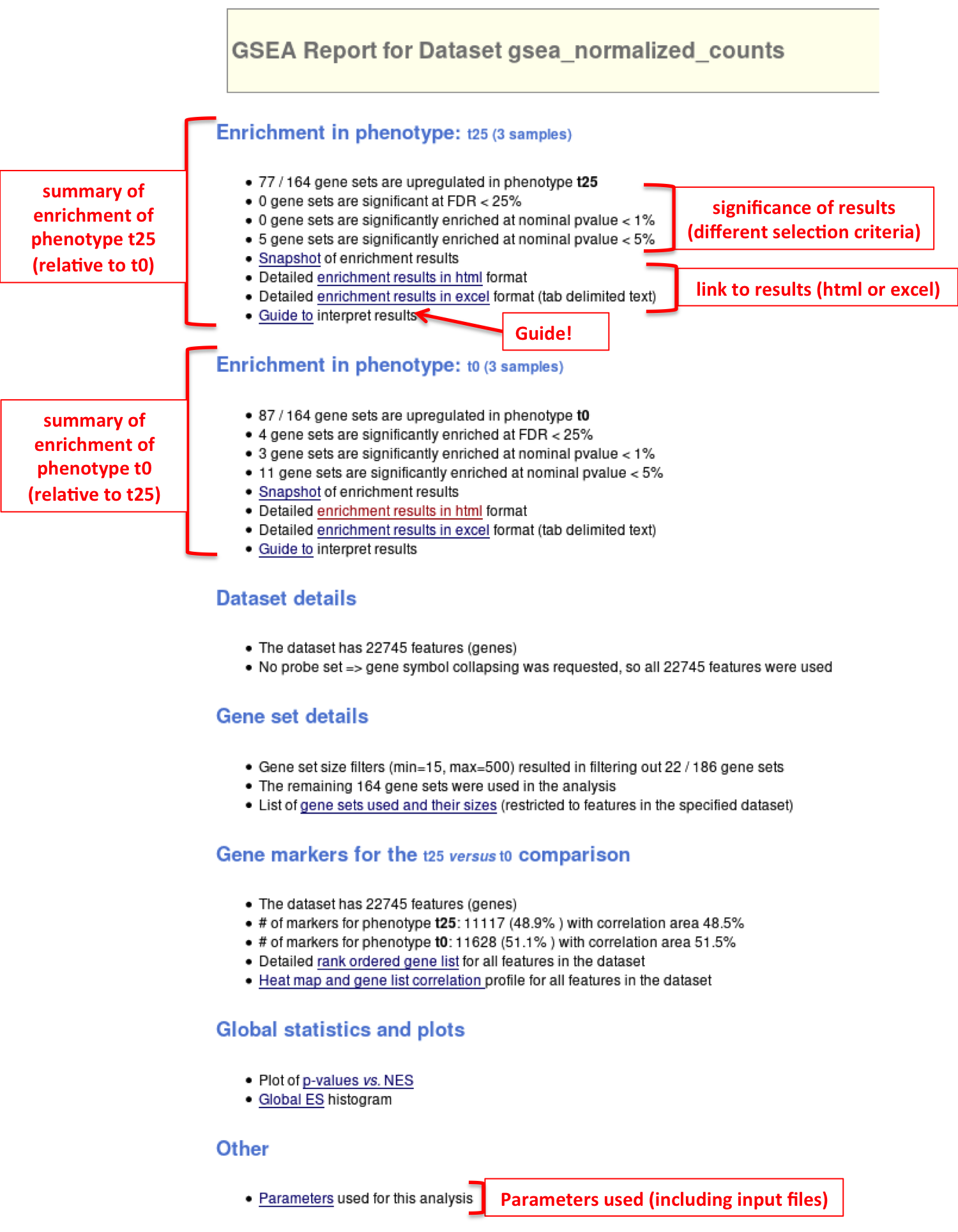
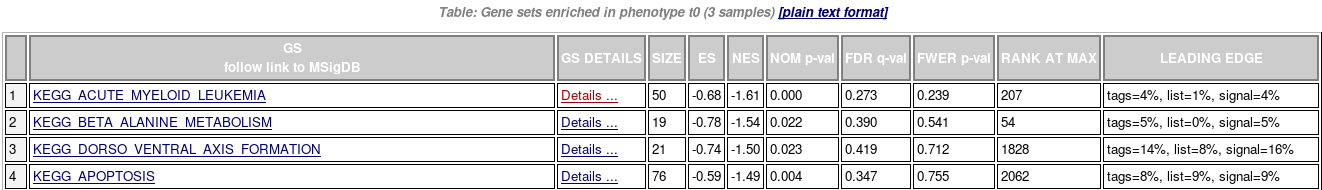
• Enrichments results in html

• Details for one gene set
  • Summary of enrichment: phenotype, stats (Nominal p-value, FDR q-value, FWER p-value), enrichment scores (ES and Normalized ES)
  • Enrichment plot

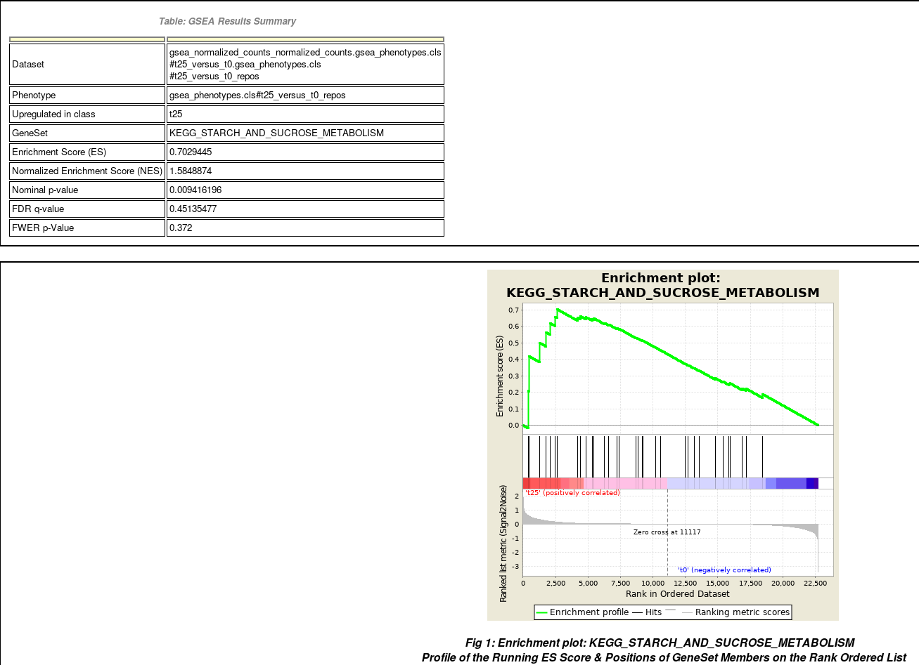
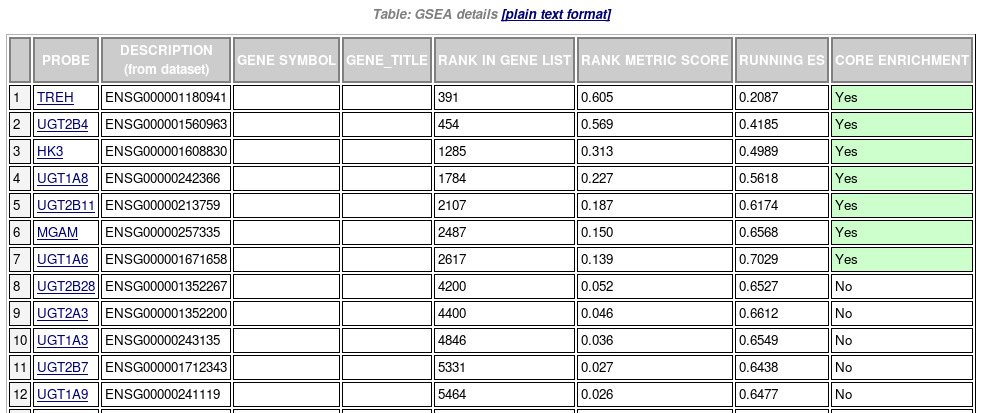
Table of genes: ranking, individual enrichment scores, core enrichment Yes/No.

From GSEA documentation, regarding core enrichment genes: “Genes with a Yes value in this column contribute to the leading-edge subset within the gene set. This is the subset of genes that contributes most to the enrichment result.”

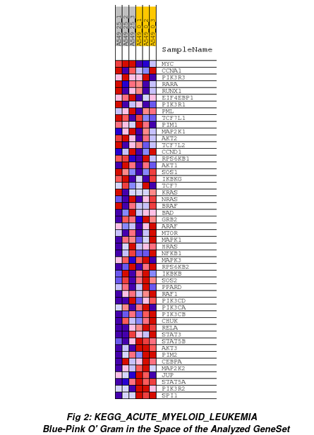
Heatmap of all genes from that gene set (ranked by GSEA) for each sample:

Suggestions for GSEA:

• Selection of pathways / gene sets: select the lowest FDR first.
• If you are looking for genes to validate on certain pathways:
  • It is better if those genes belong to the core enrichment.
  • It is also good to go back to the differential expression analysis table and make sure that their adjusted-value is low.
• You can also upload your own gene sets (for example a gene signature taken from a specific paper) to test against your list of genes, using one of the GSEA gene set database formats.

---